.ipynb .pdf

repository suggest edit

Binder

Contents

Tutorial 2 - Spatial Network analysis

Attention

Finnish university students are encouraged to use the CSC Notebooks platform.

Others can follow the lesson interactively using Binder. Check the rocket icon on the top of this page.

Lesson objectives

This tutorial focuses on spatial networks and learn how to construct a routable directed graph for Networkx and find shortest paths along the given street network based on travel times or distance by car. In addition, we will learn how to calculate travel times from a single source into all nodes in the graph.

Tutorial

In this tutorial we will focus on a network analysis methods that relate to way-finding. Finding a shortest path from A to B using a specific street network is a very common spatial analytics problem that has many practical applications.

Python provides easy to use tools for conducting spatial network analysis. One of the easiest ways to start is to use a library called Networkx which is a Python module that provides a lot tools that can be used to analyze networks on various different ways. It also contains algorithms such as Dijkstra’s algorithm or A* algoritm that are commonly used to find shortest paths along transportation network.

Next, we will learn how to do spatial network analysis in practice.

Typical workflow for routing

If you want to conduct network analysis (in any programming language) there are a few basic steps that typically needs to be done before you can start routing. These steps are:

1. Retrieve data (such as street network from OSM or Digiroad + possibly transit data if routing with PT).

2. Modify the network by adding/calculating edge weights (such as travel times based on speed limit and length of the road segment).

3. Build a routable graph for the routing tool that you are using (e.g. for NetworkX, igraph or OpenTripPlanner).

4. Conduct network analysis (such as shortest path analysis) with the routing tool of your choice.

1. Retrieve data

As a first step, we need to obtain data for routing. Pyrosm library makes it really easy to retrieve routable networks from OpenStreetMap (OSM) with different transport modes (walking, cycling and driving).

• Let’s first extract OSM data for Helsinki that are walkable. In pyrosm, we can use a function called osm.get_network() which retrieves data from OpenStreetMap. It is possible to specify what kind of roads should be retrieved from OSM with network_type -parameter (supports walking, cycling, driving).

from pyrosm import OSM, get_data
import geopandas as gpd
import pandas as pd
import networkx as nx

# We will use test data for Helsinki that comes with pyrosm
osm = OSM(get_data("helsinki_pbf"))

# Parse roads that can be driven by car
roads = osm.get_network(network_type="driving")
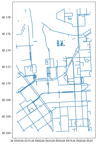
roads.plot(figsize=(10,10))

<AxesSubplot:>

roads.head(2)

	access	area	bicycle	bridge	cycleway	foot	footway	highway	int_ref	lanes	...	surface	tunnel	width	id	timestamp	version	tags	osm_type	geometry	length
0	None	None	None	None	None	None	None	unclassified	None	2	...	paved	None	None	4236349	1380031970	21	{"name:fi":"Erottajankatu","name:sv":"Skillnad...	way	MULTILINESTRING ((24.94327 60.16651, 24.94337 ...	14.0
1	None	None	None	None	None	None	None	unclassified	None	2	...	paved	None	None	4243035	1543430213	12	{"name:fi":"Korkeavuorenkatu","name:sv":"H\u00...	way	MULTILINESTRING ((24.94567 60.16767, 24.94567 ...	51.0

2 rows × 30 columns

Okay, now we have drivable roads as a GeoDataFrame for the city center of Helsinki. If you look at the GeoDataFrame (scroll to the right), we can see that pyrosm has also calculated us the length of each road segment (presented in meters). The geometries are presented here as MultiLineString objects. From the map above we can see that the data also includes short pieces of roads that do not lead to anywhere (i.e. they are isolated). This is a typical issue when working with real-world data such as roads. Hence, at some point we need to take care of those in someway (remove them (typical solution), or connect them to other parts of the network).

In OSM, the information about the allowed direction of movement is stored in column oneway. Let’s take a look what kind of values we have in that column:

roads["oneway"].unique()

array(['yes', None, 'no'], dtype=object)

As we can see the unique values in that column are "yes", "no" or None. We can use this information to construct a directed graph for routing by car. For walking and cycling, you typically want create a bidirectional graph, because the travel is typically allowed in both directions at least in Finland. Notice, that the rules vary by country, e.g. in Copenhagen you have oneway rules also for bikes but typically each road have the possibility to travel both directions (you just need to change the side of the road if you want to make a U-turn). Column maxspeed contains information about the speed limit for given road:

roads["maxspeed"].unique()

array(['30', '40', None, '20', '10', '5', '50'], dtype=object)

As we can see, there are also None values in the data, meaning that the speed limit has not been tagged for some roads. This is typical, and often you need to fill the non existing speed limits yourself. This can be done by taking advantage of the road class that is always present in column highway:

roads["highway"].unique()

array(['unclassified', 'residential', 'secondary', 'service', 'tertiary',
       'primary', 'primary_link', 'cycleway', 'footway', 'tertiary_link',
       'pedestrian', 'trail', 'crossing'], dtype=object)

Based on these values, we can make assumptions that e.g. residential roads in Helsinki have a speed limit of 30 kmph. Hence, this information can be used to fill the missing values in maxspeed. As we can see, the current version of the pyrosm tool seem to have a bug because some non-drivable roads were also leaked to our network (e.g. footway, cycleway). If you notice these kind of issues with any of the libraries that you use, please notify the developers by raising an Issue in GitHub. This way, you can help improving the software. For this given problem, an issue has already been raised so you don’t need to do it again (it’s always good to check if a related issue exists in GitHub before adding a new one).

Okay, but how can we make a routable graph out of this data of ours? Let’s remind us about the basic elements of a graph that we went through in the lecture slides:

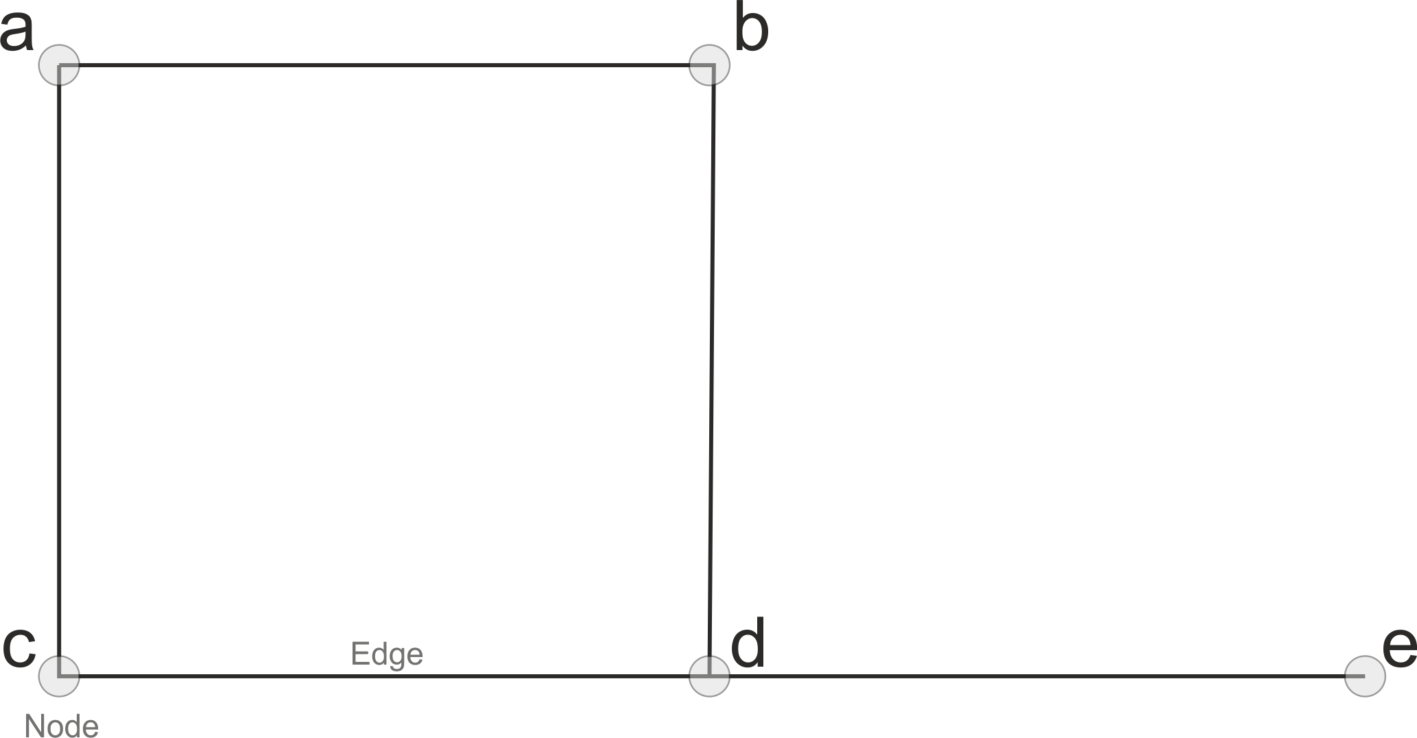
So to be able to create a graph we need to have nodes and edges. Now we have a GeoDataFrame of edges, but where are those nodes? Well they are not yet anywhere, but with pyrosm we can easily retrieve the nodes as well by specifying nodes=True, when parsing the streets:

# Parse nodes and edges
nodes, edges = osm.get_network(network_type="driving", nodes=True)

# Plot the data
ax = edges.plot(figsize=(10,10), color="gray", lw=1.0)
ax = nodes.plot(ax=ax, color="red", markersize=2)

# Zoom in to take a closer look
#ax.set_xlim([24.9375, 24.945])
ax.set_ylim([60.17, 60.173])

(60.17, 60.173)

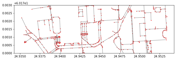
Okay, as we can see now we have both the roads (i.e. edges) and the nodes that connect the street elements together (in red) that are typically intersections. However, we can see that many of the nodes are in locations that are clearly not intersections. This is intented behavior to ensure that we have full connectivity in our network. We can at later stage clean and simplify this network by merging all roads that belong to the same link (i.e. street elements that are between two intersections) which also reduces the size of the network.

Note

In OSM, the street topology is typically not directly suitable for graph traversal due to missing nodes at intersections which means that the roads are not splitted at those locations. The consequence of this, is that it is not possible to make a turn if there is no intersection present in the data structure. Hence, pyrosm will separate all road segments/geometries into individual rows in the data.

Let’s take a look what our nodes data look like:

nodes.head()

	lon	lat	tags	timestamp	version	changeset	id	geometry
0	24.943271	60.166514	None	1390926206	2	0	1372477605	POINT (24.94327 60.16651)
1	24.943365	60.166444	{'highway': 'crossing', 'crossing': 'traffic_s...	1383915357	6	0	292727220	POINT (24.94337 60.16644)
2	24.943403	60.166408	None	1374595731	1	0	2394117042	POINT (24.94340 60.16641)
3	24.945668	60.167668	{'highway': 'crossing', 'crossing': 'uncontrol...	1290714658	5	0	296250563	POINT (24.94567 60.16767)
4	24.945671	60.167630	{'traffic_calming': 'divider'}	1354578076	1	0	2049084195	POINT (24.94567 60.16763)

As we can see, the nodes GeoDataFrame contains information about the coordinates of each node as well as a unique id for each node. These id values are used to determine the connectivity in our network. Hence, pyrosm has also added two columns to the edges GeoDataFrame that specify from and to ids for each edge. Column u contains information about the from-id and column v about the to-id accordingly:

# Check last four columns
edges.iloc[:5,-4:]

	geometry	u	v	length
0	LINESTRING (24.94327 60.16651, 24.94337 60.16644)	1372477605	292727220	9.370
1	LINESTRING (24.94337 60.16644, 24.94340 60.16641)	292727220	2394117042	4.499
2	LINESTRING (24.94567 60.16767, 24.94567 60.16763)	296250563	2049084195	4.174
3	LINESTRING (24.94567 60.16763, 24.94569 60.16744)	2049084195	60072359	21.692
4	LINESTRING (24.94569 60.16744, 24.94571 60.16726)	60072359	6100704327	19.083

We can see that the geometries are now stored as LineString instead of MultiLineString. At this point, we can fix the issue related to having some pedestrian roads in our network. We can do this by removing all edges from out GeoDataFrame that have highway value in 'cycleway', 'footway', 'pedestrian', 'trail', 'crossing':

edges = edges.loc[~edges["highway"].isin(['cycleway', 'footway', 'pedestrian', 'trail', 'crossing'])]
edges.plot()

<AxesSubplot:>

Now we can see, that some of the isolated edges were removed from the data. The character ~ (tilde) in the command above is a negation operator that is handy if you want to e.g. remove some rows from your GeoDataFrame based on criteria such as we used here.

2. Modify the data

At this stage, we have the necessary components to build a routable graph (nodes and edges) based on distance. However, in real life the network distance is not the best cost metric to use, because the shortest path (based on distance) is not necessarily always the optimal route in terms of travel time. Time is typically the measure that people value more (plus it is easier to comprehend), so at this stage we want to add a new cost attribute to our edges GeoDataFrame that converts the metric distance information to travel time (in seconds) based on following formula:

• <distance-in-meters> / (<speed-limit-kmph> / 3.6)

Before we can do this calculation, we need to ensure that all rows in maxspeed column have information about the speed limit. Let’s check the value counts of the column and also include information about the NaN values with dropna parameter:

# Count values
edges["maxspeed"].value_counts(dropna=False)

30     1110
NaN     628
40      422
10       50
20       36
5        21
50        2
Name: maxspeed, dtype: int64

As we can see, the rows which do not contain information about the speed limit is the second largest group in our data. Hence, we need to apply a criteria to fill these gaps. We can do this based on following “rule of thumb” criteria in Finland (notice that these vary country by country):

Road class	Speed limit within urban region	Speed limit outside urban region
motorway	100	120
motorway_link	80	80
trunk	60	100
trunk_link	60	60
primary	50	80
primary_link	50	50
secondary	50	50
secondary_link	50	50
tertiary	50	60
tertiary_link	50	50
unclassified	50	80
unclassified_link	50	50
residential	50	80
living_street	20	NA
service	30	NA
other	50	80

For simplicity, we can consider that all the roads in Helsinki Region follows the within urban region speed limits, although this is not exactly true (the higher speed limits start somewhere at the outer parts of the city region). For making the speed limit values more robust / correct, you could use data about urban/rural classification which is available in Finland from Finnish Environment Institute. Let’s first convert our maxspeed values to integers using astype() method:

edges["maxspeed"] = edges["maxspeed"].astype(float).astype(pd.Int64Dtype())
edges["maxspeed"].unique()

<IntegerArray>
[30, 40, <NA>, 20, 10, 5, 50]
Length: 7, dtype: Int64

As we can see, now the maxspeed values are stored in integer format inside an IntegerArray, and the None values were converted into pandas.NA objects that are assigned with <NA>. Now we can create a function that returns a numeric value for different road classes based on the criteria in the table above:

def road_class_to_kmph(road_class):
    """
    Returns a speed limit value based on road class, 
    using typical Finnish speed limit values within urban regions.
    """
    if road_class == "motorway":
        return 100
    elif road_class == "motorway_link":
        return 80
    elif road_class in ["trunk", "trunk_link"]:
        return 60
    elif road_class == "service":
        return 30
    elif road_class == "living_street":
        return 20
    else:
        return 50

Now we can apply this function to all rows that do not have speed limit information:

# Separate rows with / without speed limit information 
mask = edges["maxspeed"].isnull()
edges_without_maxspeed = edges.loc[mask].copy()
edges_with_maxspeed = edges.loc[~mask].copy()

# Apply the function and update the maxspeed
edges_without_maxspeed["maxspeed"] = edges_without_maxspeed["highway"].apply(road_class_to_kmph)
edges_without_maxspeed.head(5).loc[:, ["maxspeed", "highway"]]

	maxspeed	highway
30	30	service
47	30	service
48	30	service
49	30	service
50	30	service

Okay, as we can see now the maxspeed value have been updated according our criteria, and e.g. the service road class have been given the speed limit 30 kmph. Now we can recreate the edges GeoDataFrame by combining the two frames:

edges = edges_with_maxspeed.append(edges_without_maxspeed)
edges["maxspeed"].unique()

<IntegerArray>
[30, 40, 20, 10, 5, 50]
Length: 6, dtype: Int64

Great, now all of our edges have information about the speed limit. We can also visualize them:

# Convert the value into regular integer Series (the plotting requires having Series instead of IntegerArray) 
edges["maxspeed"] = edges["maxspeed"].astype(int)
ax = edges.plot(column="maxspeed", figsize=(10,10), legend=True)

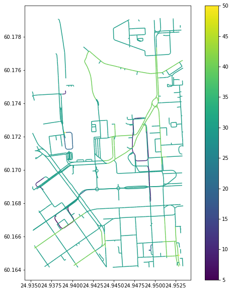
Finally, we can calculate the travel time in seconds using the formula we saw earlier and add that as a new cost attribute for our network:

edges["travel_time_seconds"] = edges["length"] / (edges["maxspeed"]/3.6)
edges.iloc[0:10, -4:]

	u	v	length	travel_time_seconds
0	1372477605	292727220	9.370	1.12440
1	292727220	2394117042	4.499	0.53988
2	296250563	2049084195	4.174	0.50088
3	2049084195	60072359	21.692	2.60304
4	60072359	6100704327	19.083	2.28996
5	6100704327	296250223	6.027	0.72324
6	264015226	25345665	9.644	1.15728
7	25345665	296248024	7.016	0.84192
8	296248024	426911766	4.137	0.49644
9	426911766	60072364	21.132	2.53584

Excellent! Now our GeoDataFrame has all the information we need for creating a graph that can be used to conduct shortest path analysis based on length or travel time. Notice that here we assume that the cars can drive with the same speed as what the speed limit is. Considering the urban dynamics and traffic congestion, this assumption might not hold, but for simplicity, we assume so in this tutorial.

3. Build a directed graph

Now as we have calculated the travel time for our edges. We still need to convert our nodes and edges into a directed graph, so that we can start using it for routing. There are easy-to-use functionalities for doing this in pyrosm and osmnx, but we will do this manually by ourselves, so that you understand what is going on under the hood.

First of all, we need to take care that our edges correctly represent a directed network. This means that we need to look at the values in oneway column and modify our edges based on the rules set in that column. If the oneway is 'yes', it means that the street can be driven only to one direction, and if it is None or has a value "no", then that road can be driven to both directions. This means that we need to make new duplicate edge and reversing the from-id and to-id values in the u and v columns. In addition, value -1 in the oneway column means that the road can only be driven to one direction but against the digitization direction. In such cases, we need to flip the to-id (u) and from-id (u) values so that the directionality in the graph is correctly specified. Let’s first check what kind of values we have in the oneway column:

edges["oneway"].unique()

array(['yes', None, 'no'], dtype=object)

Okay, in this small sample of ours, we do not seem to have any reversed oneway edges (-1) which makes things a bit easier for us, as we do not need to swap the from and to-ids. But we still need to ensure that our data is presented in such a way that a directed graph can be made out of it. Hence, we need to:

1. Separate one-way and two-way streets

2. For two-way streets, we need to create edges to opposite direction

3. (For one-way streets, we do not need to do anything in this case because there weren’t any -1 values)

Let’s start from step 1 and separate the one-way and two-way streets:

oneway = edges.loc[edges["oneway"]=="yes"].copy().reset_index()
twoway = edges.loc[edges["oneway"].isin(["no", None])].copy().reset_index()

Let’s ensure that we have successfully selected all rows in our data. Doing these kind of checks e.g. with assert is always good to do, when you e.g. split your dataset into two groups:

assert len(oneway) + len(twoway) == len(edges)

Okay, we seem to be okay because the assert did not raise any errors. Next, we want to continue processing the twoway edges and create edges for other direction. Let’s start by creating a copy out of the twoway edges for opposite direction:

# Make a copy out of twoway edges
opposite_direction = twoway.copy()

# Now the frames should be identical
pd.testing.assert_frame_equal(twoway, opposite_direction)

Okay good, now we have an identical copy of the twoway edges. Next, to change the direction of the edges in opposite_direction we simply need to specify that all the values in u becomes v, and all the values in v becomes u. The easiest way of achieving this is simply by renaming the columns because we do not need to do anything else with the values:

opposite_direction = opposite_direction.rename(columns={"u": "v", "v": "u"})

# Let's check the changes
print(twoway.loc[0, ["u", "v"]])
print()
print(opposite_direction.loc[0, ["u", "v"]])

u     296250563
v    2049084195
Name: 0, dtype: object

u    2049084195
v     296250563
Name: 0, dtype: object

Okay, as we can see now the from/to ids of the edges have been swapped, which is visible at row index 0 (the Name here tells us about the index). Now we need to merge all these edges together into a single GeoDataFrame:

directed_edges = pd.concat([oneway, twoway, opposite_direction], ignore_index=True)
print("Original edge count:", len(edges))
print("Directed edge count:", len(directed_edges))

Original edge count: 2269
Directed edge count: 3387

As we can see, now the number of edges has increased because we needed to create those opposite-direction extra edges for the two-way streets. Now we are ready to convert this GeoDataFrame into a graph! In this tutorial, we will use NetworkX library for routing. We need to convert our nodes and directed_edges into a data structures that can be ingested by the networkx.MultiDiGraph object. Basically, we need to parse edge and node attributes from our GeoDataFrames, and create an edge list having information about the from-ids and to-ids.

NetworkX uses a “dictionary of dictionaries of dictionaries” as the basic network data structure. This allows fast lookup with reasonable storage for large sparse networks. Let’s start by converting the edge and nodes attribute information into a dictionary format:

# Specify "id" as the index for nodes
nodes = nodes.set_index("id", drop=False)
nodes = nodes.rename_axis([None])

edge_attributes = directed_edges.to_dict(orient="index")
node_attributes = nodes.to_dict(orient="index")

# Now the edges are inside a dictionary where the index number if the key, 
# and as value we have another dictionary with all the attribute values for given row
edge_attributes[0]

{'index': 0,
 'access': None,
 'area': None,
 'bicycle': None,
 'bridge': None,
 'cycleway': None,
 'foot': None,
 'footway': None,
 'highway': 'unclassified',
 'int_ref': None,
 'lanes': '2',
 'lit': 'yes',
 'maxspeed': 30,
 'motorcar': None,
 'motor_vehicle': None,
 'name': 'Erottajankatu',
 'oneway': 'yes',
 'overtaking': None,
 'psv': None,
 'service': None,
 'segregated': None,
 'surface': 'paved',
 'tunnel': None,
 'width': None,
 'id': 4236349,
 'timestamp': 1380031970,
 'version': 21,
 'tags': '{"name:fi":"Erottajankatu","name:sv":"Skillnadsgatan","parking:lane:both":"no_stopping","parking:condition:reason":"junction"}',
 'osm_type': 'way',
 'geometry': <shapely.geometry.linestring.LineString at 0x7fd5d7ed8940>,
 'u': 1372477605,
 'v': 292727220,
 'length': 9.37,
 'travel_time_seconds': 1.1243999999999998}

Networkx wants the node attributes to be in a list of tuples such as [(node-id-0, dict_of_node_attributes_at_0), (node-id-1, dict_of_node_attributes_at_1)]. Let’s do this:

node_attributes = [(k, v) for k, v in node_attributes.items()]

node_attributes[0]

(1372477605,
 {'lon': 24.9432708,
  'lat': 60.1665138,
  'tags': None,
  'timestamp': 1390926206,
  'version': 2,
  'changeset': 0,
  'id': 1372477605,
  'geometry': <shapely.geometry.point.Point at 0x7fd5d7ee54c0>})

Okay, now the node attributes follow the specified structure. At this point, our edge and node attributes are ready. Next, we need to create an edge list that specify the network structure of the MultiDiGraph (i.e. how the nodes are connected together). This can be done easily by iterating over the edges and adding the u and v column information and edge attributes into a list.

node_ids = nodes["id"].to_list()

edge_list = []

for i in range(0, len(directed_edges)):
    e_attrib = edge_attributes[i]
    from_node_id = e_attrib["u"]
    to_node_id = e_attrib["v"]
    
    # Both from_node_id and to_node_id needs to exist in our nodes 
    if from_node_id not in node_ids:
        print("Did not find from-node", from_node_id)
        continue
    if to_node_id not in node_ids:
        print("Did not find to-node", to_node_id)
        continue
    
    edge = [from_node_id, to_node_id, e_attrib]
    edge_list.append(edge)

# Create the graph
graph = nx.MultiDiGraph()
graph.add_nodes_from(node_attributes)
graph.add_edges_from(edge_list);

# What do we have?
graph

<networkx.classes.multidigraph.MultiDiGraph at 0x7fd5d82a73a0>

Awesome, now we have created a NetworkX MultiDigraph object that we can use for doing routing. This hopefully gives you an idea how it is possible to create a routable graph from street network. Similar approach can be used for constructing routable graphs from many different data sources, such as Digiroad which is the national street database in Finland. Naturally the code needs to be adjusted to reflect the data structure of Digiroad or any other street network data that you want to use. You need to have some information about the allowed driving directions as well as the from and to-ids for each edge. These ids are not necessarily present in the data by default. In such cases, you can create your own ids e.g. based on vertices of the edge geometries (i.e. the x-y coordinates of the vertices can be used to create a unique node-id).

Naturally, if you are using OpenStreetMap data, you do not necessarily need to build graphs yourself, because pyrosm library (as well as OSMnx) contains functions that does all this work for you. Let’s see how we can create a routable NetworkX graph using pyrosm:

G = osm.to_graph(nodes, edges, graph_type="networkx")
G

<networkx.classes.multidigraph.MultiDiGraph at 0x7fd5d8081640>

Now we have a similar routable graph, but pyrosm actually does some additional steps in the background. By default, pyrosm cleans all unconnected edges from the graph and only keeps edges that can be reached from every part of the network. In addition, pyrosm automatically modifies the graph attribute information in a way that they are compatible with OSMnx that provides many handy functionalities to work with graphs. Such as plotting an interactive map based on the graph:

import osmnx as ox 
ox.plot_graph_folium(G)

Make this Notebook Trusted to load map: File -> Trust Notebook

4. Routing with NetworkX

Now we have everything we need to start routing with NetworkX (based on driving distance or travel time). But first, let’s again go through some basics about routing.

Basic logic in routing

Most (if not all) routing algorithms work more or less in a similar manner. The basic steps for finding an optimal route from A to B, is to:

1. Find the nearest node for origin location * (+ get info about its node-id and distance between origin and node)

2. Find the nearest node for destination location * (+ get info about its node-id and distance between origin and node)

3. Use a routing algorithm to find the shortest path between A and B

4. Retrieve edge attributes for the given route(s) and summarize them (can be distance, time, CO2, or whatever)

* in more advanced implementations you might search for the closest edge

This same logic should be applied always when searching for an optimal route between a single origin to a single destination, or when calculating one-to-many -type of routing queries (producing e.g. travel time matrices).

Find the optimal route between two locations

Next, we will learn how to find the shortest path between two locations using Dijkstra’s algorithm.

First, let’s find the closest nodes for two locations that are located in the area. OSMnx provides a handly function for geocoding an address ox.geocode(). We can use that to retrieve the x and y coordinates of our origin and destination.

# OSM data is in WGS84 so typically we need to use lat/lon coordinates when searching for the closest node

# Origin
orig_address = "Simonkatu 3, Helsinki"
orig_y, orig_x = ox.geocode(orig_address)  # notice the coordinate order (y, x)!

# Destination
dest_address = "Unioninkatu 33, Helsinki"
dest_y, dest_x = ox.geocode(dest_address) 

print("Origin coords:", orig_x, orig_y)
print("Destination coords:", dest_x, dest_y)

Origin coords: 24.9360071 60.1696202
Destination coords: 24.950513 60.1732067

Okay, now we have coordinates for our origin and destination.

Find the nearest nodes

Next, we need to find the closest nodes from the graph for both of our locations. For calculating the closest point we use here 'haversine' formula to get the distance in meters (with return_dist=True).

# 1. Find the closest nodes for origin and destination
orig_node_id, dist_to_orig = ox.get_nearest_node(G, point=(orig_y, orig_x), method='haversine', return_dist=True)
dest_node_id, dist_to_dest = ox.get_nearest_node(G, point=(dest_y, dest_x), method='haversine', return_dist=True)

print("Origin node-id:", orig_node_id, "and distance:", dist_to_orig, "meters.")
print("Destination node-id:", dest_node_id, "and distance:", dist_to_dest, "meters.")

Origin node-id: 659998487 and distance: 27.888258768172825 meters.
Destination node-id: 1012323567 and distance: 0.0 meters.

Now we are ready to start the actual routing with NetworkX.

Find the fastest route by distance / time

Now we can do the routing and find the shortest path between the origin and target locations by using the dijkstra_path() function of NetworkX. For getting only the cumulative cost of the trip, we can directly use a function dijkstra_path_length() that returns the travel time without the actual path.

With weight -parameter we can specify the attribute that we want to use as cost/impedance. We have now three possible weight attributes available: 'length' and 'travel_time_seconds'.

• Let’s first calculate the routes between locations by walking and cycling, and also retrieve the travel times

# Calculate the paths by walking and cycling
metric_path = nx.dijkstra_path(G, source=orig_node_id, target=dest_node_id, weight='length')
time_path = nx.dijkstra_path(G, source=orig_node_id, target=dest_node_id, weight='travel_time_seconds')

# Get also the actual travel times (summarize)
travel_length = nx.dijkstra_path_length(G, source=orig_node_id, target=dest_node_id, weight='length')
travel_time = nx.dijkstra_path_length(G, source=orig_node_id, target=dest_node_id, weight='travel_time_seconds')

Okay, that was it! Let’s now see what we got as results by visualizing the results.

For visualization purposes, we can use a handy function again from OSMnx called ox.plot_graph_route() (for static) or ox.plot_route_folium() (for interactive plot).

• Let’s first make static maps

# Shortest path based on distance
fig, ax = ox.plot_graph_route(G, metric_path)

# Add the travel time as title
ax.set_xlabel("Shortest path distance {t: .1f} meters.".format(t=travel_length))

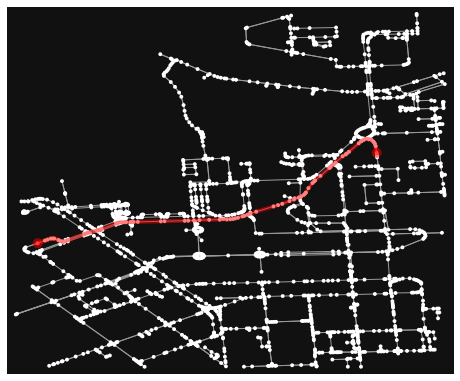
Text(0.5, 51.0, 'Shortest path distance  1081.7 meters.')

fig, ax = ox.plot_graph_route(G, time_path)

# Add the travel time as title
ax.set_xlabel("Travel time {t: .1f} minutes.".format(t=travel_time/60))

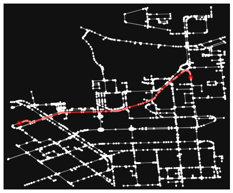
Text(0.5, 51.0, 'Travel time  2.0 minutes.')

Great! Now we have successfully found the optimal route between our origin and destination and we also have estimates about the travel time that it takes to travel between the locations by walking and cycling. As we can see, the route for both travel modes is exactly the same which is natural, as the only thing that changed here was the constant travel speed.

• Let’s still finally see an example how you can plot a nice interactive map out of our results with OSMnx:

ox.plot_route_folium(G, time_path, popup_attribute='travel_time_seconds')

Make this Notebook Trusted to load map: File -> Trust Notebook

Calculate travel times from one to many locations

When trying to understand the accessibility of a specific location, you typically want to look at travel times between multiple locations (one-to-many) or use isochrones (travel time contours).

• Let’s see how we can calculate travel times from the origin node, to all other nodes in our graph using NetworkX function single_source_dijkstra_path_length():

# Calculate walk travel times originating from one location
travel_times = nx.single_source_dijkstra_path_length(G, source=orig_node_id, weight='travel_time_seconds')

# What did we get?
#travel_times

As we can see, the result is a dictionary where we have the node_id as keys and the travel time as values.

For visualizing this information, we need to join this data with the nodes. For doing this, we can first convert the result to DataFrame and then we can easily merge the information with the nodes GeoDataFrame.

import pandas as pd
# Convert to DataFrame and add column names
travel_times_df = pd.DataFrame([list(travel_times.keys()), list(travel_times.values())]).T
travel_times_df.columns = ['node_id', 'travel_time']

# What do we have now?
travel_times_df.head()

	node_id	travel_time
0	6.599985e+08	0.00000
1	3.236097e+09	7.62948
2	3.236097e+09	10.28592
3	2.960448e+08	11.32884
4	3.236097e+09	11.90532

Great! Now we have the travel times from origin to all other nodes in the graph.

• Let’s finally merge the data with the nodes GeoDataFrame and visualize the results

# Check the nodes
nodes.head()

	lon	lat	tags	timestamp	version	changeset	id	geometry
1372477605	24.943271	60.166514	None	1390926206	2	0	1372477605	POINT (24.94327 60.16651)
292727220	24.943365	60.166444	{'highway': 'crossing', 'crossing': 'traffic_s...	1383915357	6	0	292727220	POINT (24.94337 60.16644)
2394117042	24.943403	60.166408	None	1374595731	1	0	2394117042	POINT (24.94340 60.16641)
296250563	24.945668	60.167668	{'highway': 'crossing', 'crossing': 'uncontrol...	1290714658	5	0	296250563	POINT (24.94567 60.16767)
2049084195	24.945671	60.167630	{'traffic_calming': 'divider'}	1354578076	1	0	2049084195	POINT (24.94567 60.16763)

As we can see, the node_id in the nodes GeoDataFrame can be found from the index of the gdf as well as from the column osmid.

• Let’s merge these two datasets:

# Merge the datasets
nodes_viz = nodes.merge(travel_times_df, left_on='id', right_on='node_id')

# Check
nodes_viz.head()

	lon	lat	tags	timestamp	version	changeset	id	geometry	node_id	travel_time
0	24.943271	60.166514	None	1390926206	2	0	1372477605	POINT (24.94327 60.16651)	1.372478e+09	79.60704
1	24.943365	60.166444	{'highway': 'crossing', 'crossing': 'traffic_s...	1383915357	6	0	292727220	POINT (24.94337 60.16644)	2.927272e+08	80.73144
2	24.943403	60.166408	None	1374595731	1	0	2394117042	POINT (24.94340 60.16641)	2.394117e+09	81.27132
3	24.945668	60.167668	{'highway': 'crossing', 'crossing': 'uncontrol...	1290714658	5	0	296250563	POINT (24.94567 60.16767)	2.962506e+08	103.99572
4	24.945671	60.167630	{'traffic_calming': 'divider'}	1354578076	1	0	2049084195	POINT (24.94567 60.16763)	2.049084e+09	103.49484

Okay, now we have also the travel times associated for each node.

• Let’s visualize this:

from shapely.geometry import Point

# Make a GeoDataFrame for the origin point so that we can visualize it
orig = gpd.GeoDataFrame({'geometry': [Point(orig_x, orig_y)]}, index=[0], crs='epsg:4326')

# Plot the results with edges and the origin point (green)
ax = edges.plot(lw=0.5, color='gray', zorder=0, figsize=(10,10))
ax = nodes_viz.plot('travel_time', ax=ax, cmap='RdYlBu', scheme='natural_breaks', k=5, markersize=30, legend=True)
ax = orig.plot(ax=ax, markersize=100, color='green')

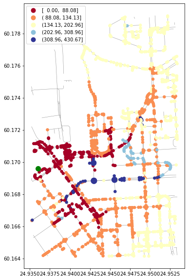
Okay, as we can see now we have quickly calculated the travel times for each node in the graph using a single call.

If you would have for example a predefined grid, you could find the nearest node for each grid centroid to produce a more matrix-like result.

Alternative approach - Ego graph

Alternatively, it is possible to directly set a specific time limit and restrict how long the graph is travelled from the origin, and return that subgraph for the user.

• Let’s see an example:

# Take a subgraph until 1 minutes by driving (60 seconds)
subgraph = nx.ego_graph(G, n=orig_node_id, radius=60, distance='travel_time_seconds')
fig, ax = ox.plot_graph(subgraph)

As we can see, with this approach we can retrieve a partial graph that we could for example visualize with different colors, or e.g. subset the extent of our accessibility analysis to cover only specific range from the source.

Larger scale analysis

We can very easily create a travel time map covering larger areas as well. This is how you could calculate travel times by car from city center of Helsinki to other parts of the region:

from pyrosm import OSM, get_data
import osmnx as ox
import pandas as pd
import networkx as nx

def road_class_to_kmph(road_class):
    """
    Returns a speed limit value based on road class, 
    using typical Finnish speed limit values within urban regions.
    """
    if road_class == "motorway":
        return 100
    elif road_class == "motorway_link":
        return 80
    elif road_class in ["trunk", "trunk_link"]:
        return 60
    elif road_class == "service":
        return 30
    elif road_class == "living_street":
        return 20
    else:
        return 50
    
def assign_speed_limits(edges):
    # Separate rows with / without speed limit information 
    mask = edges["maxspeed"].isnull()
    edges_without_maxspeed = edges.loc[mask].copy()
    edges_with_maxspeed = edges.loc[~mask].copy()

    # Apply the function and update the maxspeed
    edges_without_maxspeed["maxspeed"] = edges_without_maxspeed["highway"].apply(road_class_to_kmph)
    edges = edges_with_maxspeed.append(edges_without_maxspeed)
    edges["maxspeed"] = edges["maxspeed"].astype(int)
    edges["travel_time_seconds"] = edges["length"] / (edges["maxspeed"]/3.6)
    return edges
    
# Fetch data for Helsinki
osm = OSM(get_data("helsinki"))
nodes, edges = osm.get_network(network_type="driving", nodes=True)

# Assign speed limits for missing ones based on road classs information
edges = assign_speed_limits(edges)

# Create a graph
G2 = osm.to_graph(nodes, edges, graph_type="networkx")

# Calculate travel times from central railway station
orig_address = "Rautatientori, Helsinki"
orig_y, orig_x = ox.geocode(orig_address)  # notice the coordinate order (y, x)!
orig_node_id, dist_to_orig = ox.get_nearest_node(G2, point=(orig_y, orig_x), method='haversine', return_dist=True)
travel_times = nx.single_source_dijkstra_path_length(G2, source=orig_node_id, weight='travel_time_seconds')

# Convert to DataFrame and add column names
travel_times_df = pd.DataFrame([list(travel_times.keys()), list(travel_times.values())]).T
travel_times_df.columns = ['node_id', 'travel_time']
nodes_t = nodes.merge(travel_times_df, left_on='id', right_on='node_id')

# Convert travel time to minutes
nodes_t["travel_time"] = (nodes_t["travel_time"] / 60).round(0)

# Plot the results
main_roads = edges.loc[edges["highway"].isin(["motorway", "motorway_link", "trunk", "trunk_link", "primary", "primary_link"])]
ax = main_roads.plot(lw=0.5, color='gray', zorder=3, figsize=(10,10))
ax = nodes_t.plot('travel_time', ax=ax, cmap='RdYlBu', scheme='natural_breaks', k=8, markersize=20, legend=True)

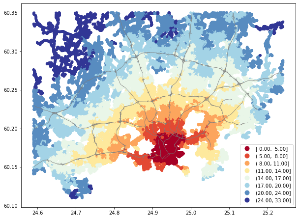
As a result, we have a map that shows travel times by driving from the central railway station of Helsinki. We can see that if assuming that you could drive according the speed limits, it would be possible to reach even the farthest parts of the region in approximately 30 minutes. Naturally this is not typically possible because of the congestion. Considering congestion in the travel times can also be taken into account by creating a model that integrates information from floating car measurements (GPS data), but it is out of scope of this tutorial.

previous

Network analytics and spatial accessibility modelling

next

Recommended readings