Tutorial 1.2 - Spatial analysis with Python

Attention

Finnish university students are encouraged to use the CSC Notebooks platform.

Others can follow the lesson interactively using Binder. Check the rocket icon on the top of this page.

In the first week, we will take a quick tour to Python’s (spatial) data science ecosystem and see how we can use some of the fundamental open source Python packages, such as:

• pandas / geopandas

• shapely

• pysal

• pyproj

• osmnx / pyrosm

• matplotlib (visualization)

As you can see, we won’t use any GIS software for doing the programming (such as ArcGIS/arcpy or QGIS), but focus on learning the open source packages that are independent from any specific software. These libraries form nowadays not only the core for modern spatial data science, but they are also fundamental parts of commercial applications used and developed by many companies around the world.

Note

If you have experience working with the Python’s spatial data science stack, this tutorial probably does not bring much new to you, but to get everyone on the same page, we will all go through this introductory tutorial.

Contents:

• Reading / writing spatial data

• Retrieving OpenStreetMap data

• Reprojections

• Spatial join

• Plotting data with matplotlib

Fundamental library: Geopandas

In this course, the most often used Python package that you will learn is geopandas. Geopandas makes it possible to work with geospatial data in Python in a relatively easy way. Geopandas combines the capabilities of the data analysis library pandas with other packages like shapely and fiona for managing spatial data. The main data structures in geopandas are GeoSeries and GeoDataFrame which extend the capabilities of Series and DataFrames from pandas. In case you wish to have additional help getting started with pandas, we recommend you to take a look lessons 5 and 6 from the openly available Geo-Python -course. The main difference between GeoDataFrames and pandas DataFrames is that a GeoDataFrame should contain (at least) one column for geometries. By default, the name of this column is 'geometry'. The geometry column is a GeoSeries which contains the geometries (points, lines, polygons, multipolygons etc.) as shapely objects.

Reading and writing spatial data

Next we will learn some of the basic functionalities of geopandas. We have a couple of GeoJSON files stored in the data folder that we will use.

We can read the data easily with read_file() -function:

import geopandas as gpd

# Filepath
fp = "data/buildings.geojson"

# Read the file
data = gpd.read_file(fp)

# How does it look?
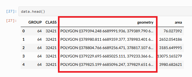
data.head()

	addr:city	addr:country	addr:housenumber	addr:housename	addr:postcode	addr:street	email	name	opening_hours	operator	...	start_date	wikipedia	id	timestamp	version	tags	osm_type	internet_access	changeset	geometry
0	Helsinki	None	29	None	00170	Unioninkatu	None	None	None	None	...	None	None	4253124	1542041335	4	None	way	None	NaN	POLYGON ((24.95121 60.16999, 24.95122 60.16988...
1	Helsinki	None	2	None	00100	Kaivokatu	ainfo@ateneum.fi	Ateneum	Tu, Fr 10:00-18:00; We-Th 10:00-20:00; Sa-Su 1...	None	...	1887	fi:Ateneumin taidemuseo	8033120	1544822447	27	{'architect': 'Theodor Höijer', 'contact:websi...	way	None	NaN	POLYGON ((24.94477 60.16982, 24.94450 60.16981...
2	Helsinki	FI	22-24	None	None	Mannerheimintie	None	Lasipalatsi	None	None	...	1936	fi:Lasipalatsi	8035238	1533831167	23	{'name:fi': 'Lasipalatsi', 'name:sv': 'Glaspal...	way	None	NaN	POLYGON ((24.93561 60.17045, 24.93555 60.17054...
3	Helsinki	None	2	None	00100	Mannerheiminaukio	None	Kiasma	Tu 10:00-17:00; We-Fr 10:00-20:30; Sa 10:00-18...	None	...	1998	fi:Kiasma (rakennus)	8042215	1553963033	30	{'name:en': 'Museum of Modern Art Kiasma', 'na...	way	None	NaN	POLYGON ((24.93682 60.17152, 24.93662 60.17150...
4	None	FI	None	None	None	None	None	None	None	None	...	None	None	15243643	1546289715	7	None	way	None	NaN	POLYGON ((24.93675 60.16779, 24.93660 60.16789...

5 rows × 34 columns

As we can see, the GeoDataFrame contains various attributes in separate columns. The geometry column contains the spatial information. We can take a look of some of the basic information about our GeoDataFrame with command:

data.info()

<class 'geopandas.geodataframe.GeoDataFrame'>
RangeIndex: 486 entries, 0 to 485
Data columns (total 34 columns):
 #   Column              Non-Null Count  Dtype   
---  ------              --------------  -----   
 0   addr:city           86 non-null     object  
 1   addr:country        57 non-null     object  
 2   addr:housenumber    88 non-null     object  
 3   addr:housename      4 non-null      object  
 4   addr:postcode       54 non-null     object  
 5   addr:street         89 non-null     object  
 6   email               2 non-null      object  
 7   name                81 non-null     object  
 8   opening_hours       8 non-null      object  
 9   operator            7 non-null      object  
 10  phone               8 non-null      object  
 11  ref                 1 non-null      object  
 12  url                 8 non-null      object  
 13  website             20 non-null     object  
 14  building            486 non-null    object  
 15  amenity             26 non-null     object  
 16  building:levels     162 non-null    object  
 17  building:material   2 non-null      object  
 18  building:min_level  4 non-null      object  
 19  height              17 non-null     object  
 20  landuse             2 non-null      object  
 21  office              5 non-null      object  
 22  shop                5 non-null      object  
 23  source              3 non-null      object  
 24  start_date          87 non-null     object  
 25  wikipedia           47 non-null     object  
 26  id                  486 non-null    int64   
 27  timestamp           486 non-null    int64   
 28  version             486 non-null    int64   
 29  tags                181 non-null    object  
 30  osm_type            486 non-null    object  
 31  internet_access     1 non-null      object  
 32  changeset           66 non-null     float64 
 33  geometry            486 non-null    geometry
dtypes: float64(1), geometry(1), int64(3), object(29)
memory usage: 129.2+ KB

From here, we can see that our data is indeed a GeoDataFrame object with 486 entries and 34 columns. You can also get descriptive statistics of your data by calling:

data.describe()

	id	timestamp	version	changeset
count	4.860000e+02	4.860000e+02	486.000000	66.0
mean	1.400780e+08	1.455829e+09	4.849794	0.0
std	1.633527e+08	9.247528e+07	4.561162	0.0
min	8.253000e+03	1.197929e+09	1.000000	0.0
25%	2.294267e+07	1.374229e+09	2.000000	0.0
50%	1.228699e+08	1.493288e+09	3.000000	0.0
75%	1.359805e+08	1.530222e+09	7.000000	0.0
max	1.042029e+09	1.555840e+09	31.000000	0.0

In this case, we didn’t have many columns with numerical data, but typically you have numeric values in your dataset and this is a good way to get a quick view how the data look like.

Naturally, as the data is spatial, we want to visualize it to understand the nature of the data better. We can do this easily with plot() method:

data.plot()

<AxesSubplot: >

Now we can see that the data indeed represents buildings (in central Helsinki).

We can also very easily make an interactive map out of this same data by using .explore() function:

data.explore()

Make this Notebook Trusted to load map: File -> Trust Notebook

Naturally we can also write this data to disk. Geopandas supports writing data to various data formats as well as to PostGIS which is the most widely used open source database for GIS. Let’s write the data as a Shapefile to the same data directory from where we read the data. When writing data to local disk you can use to_file() method that exports the data in Shapefile format by default:

# Output filepath
outfp = "data/buildings_copy.shp"
data.to_file(outfp)

/tmp/ipykernel_24597/403506898.py:3: UserWarning: Column names longer than 10 characters will be truncated when saved to ESRI Shapefile.
  data.to_file(outfp)

Retrieving data from OpenStreetMap

Now we have seen how to read spatial data from disk. OpenStreetMap (OSM) is probably the most well known and widely used spatial dataset/database in the world. Also in this course, we will use OSM data frequently. Hence, let’s see how we can retrieve data from OSM using a library called pyrosm. With pyrosm you can easily download and extract data from anywhere in the world based on OSM.PBF files that are distributed e.g. by Geofabrik. The tool aims to be an efficient way to parse OSM data covering large geographical areas (such as countries and cities), but as a downside, it is a bit limited in a sense how you can define your area of interest. With pyrosm you can extract OSM data from 654 regions in the world (covering all countries plus many city regions, see docs for further info).

Note

In case you want to extract OSM data from smaller areas, e.g. using a buffer of 2 km around a specific location, we recommend using OSMnx library, which is more flexible in terms of specifying the area of interest.

Let’s see how we can download and extract OSM data for Helsinki Region using pyrosm:

from pyrosm import OSM, get_data

# Download data for Helsinki
fp = get_data("helsinki")

# Initialize the reader object for Helsinki
osm = OSM(fp)

Downloaded Protobuf data 'Helsinki.osm.pbf' (32.95 MB) to:
'/tmp/pyrosm/Helsinki.osm.pbf'

As a first step, we downloaded the data for “Helsinki” using the get_data function, which is a helper function that automates the data downloading process and stores the data locally in a temporary folder (inside /tmp/ in this case). The next step that we did, was to initialize a reader object called OSM. The OSM takes the filepath to a given osm.pbf file as an input. Notice that at this point we didn’t yet read any data into GeoDataFrame.

OSM is a “database of the world”, hence it contains a lot of information about different things. With pyrosm you can easily extract information about:

• street networks –> osm.get_network()

• buildings –> osm.get_buildings()

• Points of Interest (POI) –> osm.get_pois()

• landuse –> osm.get_landuse()

• natural elements –> osm.get_natural()

• boundaries –> osm.get_boundaries()

Let’s see how we can read all the buildings from Helsinki Region:

buildings = osm.get_buildings()

buildings.head()

	addr:city	addr:country	addr:full	addr:housenumber	addr:housename	addr:postcode	addr:place	addr:street	email	name	...	source	start_date	wikipedia	id	timestamp	version	tags	osm_type	geometry	changeset
0	Espoo	FI	None	2	None	02150	None	Konemiehentie	None	Aalto Tietotekniikka	...	None	1998	None	4217650	0	-1	{"alt_name":"T-talo","loc_name":"Tikkitalo","n...	way	POLYGON ((24.82129 60.18718, 24.82164 60.18712...	NaN
1	None	None	None	None	None	None	None	None	None	None	...	None	None	None	4217760	0	-1	{"access":"private","parking":"multi-storey","...	way	POLYGON ((24.83776 60.18905, 24.83796 60.18938...	NaN
2	None	None	None	None	None	None	None	None	None	None	...	None	None	None	4220761	0	-1	None	way	POLYGON ((24.85599 60.20719, 24.85590 60.20719...	NaN
3	Helsinki	FI	None	5	Uimastadion	00250	None	Hammarskjöldintie	None	Uimastadion	...	None	None	None	4252923	0	-1	{"leisure":"stadium","name:en":"Swimming Stadi...	way	POLYGON ((24.93076 60.18914, 24.93067 60.18898...	NaN
4	Espoo	None	None	9	None	02150	None	Otaniementie	None	Aalto-yliopisto Harald Herlin -oppimiskeskus	...	Bing	None	None	4252948	0	-1	{"name:en":"Aalto University Harald Herlin Lea...	way	POLYGON ((24.82740 60.18514, 24.82806 60.18480...	NaN

5 rows × 40 columns

Let’s check how many buildings did we get:

len(buildings)

159411

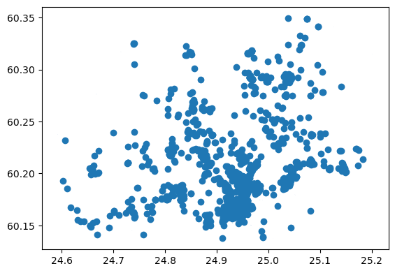
Okay, so there are more than 150 thousand buildings in the Helsinki Region. Naturally, we would like to see them on a map. Let’s plot our data using plot() (might take some time as there are many objects to plot):

buildings.plot()

<AxesSubplot: >

Great! As a result we got a map that seems to look correct.

Reprojecting data

As we can see from the previous maps that we have produced, the coordinates on the x and y axis hint that our geometries are represented in decimal degrees (WGS84). In many cases, you want to reproject your data to another CRS. Luckily, doing that is easy with geopandas. Let’s first take a look what the Coordinate Reference System (CRS) of our GeoDataFrame is. We can access the CRS information of the GeoDataFrame by accessing an attribute called crs:

buildings.crs

<Geographic 2D CRS: EPSG:4326>
Name: WGS 84
Axis Info [ellipsoidal]:
- Lat[north]: Geodetic latitude (degree)
- Lon[east]: Geodetic longitude (degree)
Area of Use:
- name: World.
- bounds: (-180.0, -90.0, 180.0, 90.0)
Datum: World Geodetic System 1984 ensemble
- Ellipsoid: WGS 84
- Prime Meridian: Greenwich

As a result, we get information about the CRS, and we can see that the data is indeed in WGS84. We can also see that the EPSG code for the CRS is 4326. We can easily reproject our data by using a method to_crs(). The easiest way to use the method is to specify the destination CRS as an EPSG code. Let’s reproject our data into EPSG 3067 which is the most widely used projected coordinate reference system used in Finland, EUREF-FIN:

projected = buildings.to_crs(epsg=3067)
projected.crs

<Derived Projected CRS: EPSG:3067>
Name: ETRS89 / TM35FIN(E,N)
Axis Info [cartesian]:
- E[east]: Easting (metre)
- N[north]: Northing (metre)
Area of Use:
- name: Finland - onshore and offshore.
- bounds: (19.08, 58.84, 31.59, 70.09)
Coordinate Operation:
- name: TM35FIN
- method: Transverse Mercator
Datum: European Terrestrial Reference System 1989 ensemble
- Ellipsoid: GRS 1980
- Prime Meridian: Greenwich

As we can see, now we have an Projected CRS as a result. To confirm the difference, let’s take a look at the geometry of the first row in our original buildings GeoDataFrame and the projected GeoDataFrame. To select a specific row in data, we can use the loc indexing:

orig_geom = buildings.loc[0, "geometry"]
projected_geom = projected.loc[0, "geometry"]

print("Orig:\n", orig_geom, "\n")
print("Proj:\n", projected_geom)

Orig:
 POLYGON ((24.8212885 60.1871792, 24.8216351 60.1871237, 24.8218626 60.1870873, 24.8218641 60.1870934, 24.8218654 60.1870987, 24.8219228 60.1870952, 24.8219186 60.1870783, 24.8219949 60.1870661, 24.8225411 60.1869791, 24.8224862 60.186896, 24.8224626 60.1868996, 24.8224423 60.1869026, 24.8223976 60.1867789, 24.8221329 60.1867998, 24.8221083 60.1867761, 24.8220836 60.1867524, 24.822336 60.186716, 24.8223039 60.186662, 24.8223248 60.1866583, 24.8223455 60.1866546, 24.8222782 60.1865828, 24.8222717 60.1865839, 24.8217847 60.1866948, 24.821782 60.1866868, 24.821718 60.1866924, 24.821721 60.1867002, 24.8217239 60.1867078, 24.8211387 60.1867604, 24.8211339 60.1867474, 24.8210732 60.1867528, 24.8210758 60.18676, 24.8210779 60.1867659, 24.8204964 60.1868181, 24.8204917 60.186805, 24.8204286 60.1868107, 24.8204316 60.1868189, 24.8204333 60.1868238, 24.8203009 60.1868357, 24.8203177 60.1868814, 24.8203355 60.18688, 24.820371 60.1869699, 24.8204695 60.186961, 24.8204728 60.18697, 24.8204764 60.18698, 24.820483 60.1869963, 24.8205879 60.1872905, 24.8206157 60.1873401, 24.8206263 60.1873572, 24.8209968 60.1872991, 24.8209637 60.1872465, 24.8209549 60.1872326, 24.821232 60.1871882, 24.8212332 60.1871951, 24.8212348 60.1872038, 24.8212923 60.1872013, 24.8212885 60.1871792)) 

Proj:
 POLYGON ((379178.3725997981 6674250.711355622, 379197.38488247665 6674243.8982704505, 379209.8642355002 6674239.429592708, 379209.9698097793 6674240.105962586, 379210.06135644973 6674240.693634215, 379213.23087879736 6674240.1989603145, 379212.9359337318 6674238.325163864, 379217.1213550152 6674236.827341885, 379247.08437153 6674226.142463202, 379243.7353683548 6674216.991336721, 379242.44014722883 6674217.435292421, 379241.3256829249 6674217.806414308, 379238.3930495286 6674204.116628114, 379223.7941370049 6674206.927641303, 379222.34318484605 6674204.334118548, 379220.8866864759 6674201.740779295, 379234.74673835706 6674197.226635681, 379232.76867210196 6674191.273522315, 379233.91383847635 6674190.823369212, 379235.0479165341 6674190.373582317, 379231.0528703418 6674182.503181034, 379230.69653105864 6674182.63753462, 379204.10322045477 6674195.875016209, 379203.9241322995 6674194.989314756, 379200.3963642038 6674195.729866023, 379200.59135121654 6674196.592752348, 379200.7800590387 6674197.433555618, 379168.52823067305 6674204.360432023, 379168.21432858787 6674202.92192481, 379164.86879993975 6674203.634204664, 379165.0394128716 6674204.431023199, 379165.17752656224 6674205.084027647, 379133.129487243 6674211.959913267, 379132.82074820774 6674210.510092845, 379129.343272631 6674211.260198221, 379129.53974651126 6674212.16761301, 379129.65201301314 6674212.710018366, 379122.35516265105 6674214.277255361, 379123.4546156952 6674219.334283684, 379124.4363452866 6674219.145831282, 379126.73506700597 6674229.089415575, 379132.16342090897 6674227.918240647, 379132.3794672409 6674228.914170477, 379132.61582245084 6674230.020881242, 379133.04166496906 6674231.823479696, 379139.9390695336 6674264.384770593, 379141.6626842505 6674269.855854501, 379142.31322685 6674271.740195557, 379162.640842104 6674264.593717466, 379160.61238877964 6674258.79833438, 379160.0734109332 6674257.266952087, 379175.27320035227 6674251.816728769, 379175.36508827226 6674252.582710911, 379175.48576795845 6674253.548355347, 379178.66449481767 6674253.16479852, 379178.3725997981 6674250.711355622))

As we can see the coordinates that form our Polygon has changed from decimal degrees to meters. Let’s see what happens if we just call the geometries:

orig_geom

projected_geom

As you can see, we can draw the geometry directly in the screen, and we can easily see the difference in the shape of the two geometries. The orig_geom and projected_geom variables contain a Shapely geometry which is Polygon in this case. We can confirm this by checking the type:

type(orig_geom)

shapely.geometry.polygon.Polygon

These shapely geometries are used as the underlying data structure in most GIS packages in Python to present geometrical information. Shapely is fundamentally a Python wrapper for GEOS which is widely used library (written in C++) under the hood of many GIS softwares such as QGIS, GDAL, GRASS, PostGIS, Google Earth etc. Currently, there is ongoing work to vectorize all the GEOS functionalities for Python and bring those eventually into Shapely which will greatly boost the performance of all geometry related operations in Python ecosystem (approaching the same efficiency as PostGIS). Some of these improvements can already be found under the hood of latest version of geopandas.

Calculating area

One thing that is quite often interesting to know when working with spatial data, is the area of the geometries. In geopandas, we can easily calculate e.g. the area for each of our buildings by:

projected["building_area"] = projected.area
projected["building_area"].describe()

count    159411.000000
mean        288.614445
std         939.708068
min           0.000000
25%          67.919331
50%         142.707799
75%         261.594790
max       84158.162750
Name: building_area, dtype: float64

We calculated the area by calling area which is the attribute containing information about areas of the buildings measured based on the map units of the data. Hence, in this case because our data is projected in Euref-FIN the units that we stored in "building_area" column are square meters. It’s important to always keep in mind the CRS when calculating areas, distances etc. with geometries.

Spatial join

A commonly needed GIS functionality, is to be able to merge information between two layers using location as the key. Hence, it is somewhat similar approach as table join but because the operation is based on geometries, it is called spatial join. Next, we will see how we can conduct a spatial join and merge information between two layers. We will read all restaurants from the OSM for Helsinki Region, and combine information from restaurants to the underlying building (restaurants typically are within buildings). We will again use pyrosm for reading the data, but this time we will use get_pois() function:

# Read Points of Interest using the same OSM reader object that was initialized earlier
restaurants = osm.get_pois(custom_filter={"amenity": ["restaurant"]})
restaurants.plot()

/home/hentenka/.conda/envs/mamba/envs/sp-test/lib/python3.9/site-packages/pyrosm/pyrosm.py:576: ShapelyDeprecationWarning: The array interface is deprecated and will no longer work in Shapely 2.0. Convert the '.coords' to a numpy array instead.
  gdf = get_poi_data(

<AxesSubplot: >

restaurants.info()

<class 'geopandas.geodataframe.GeoDataFrame'>
RangeIndex: 1573 entries, 0 to 1572
Data columns (total 37 columns):
 #   Column            Non-Null Count  Dtype   
---  ------            --------------  -----   
 0   version           1573 non-null   int8    
 1   changeset         1491 non-null   float64 
 2   timestamp         1573 non-null   int64   
 3   id                1573 non-null   int64   
 4   lat               1488 non-null   float32 
 5   tags              1521 non-null   object  
 6   lon               1488 non-null   float32 
 7   addr:city         1041 non-null   object  
 8   addr:country      380 non-null    object  
 9   addr:housenumber  1135 non-null   object  
 10  addr:housename    123 non-null    object  
 11  addr:postcode     1005 non-null   object  
 12  addr:place        1 non-null      object  
 13  addr:street       1169 non-null   object  
 14  email             209 non-null    object  
 15  name              1551 non-null   object  
 16  opening_hours     871 non-null    object  
 17  operator          68 non-null     object  
 18  phone             553 non-null    object  
 19  ref               4 non-null      object  
 20  url               29 non-null     object  
 21  website           953 non-null    object  
 22  amenity           1573 non-null   object  
 23  bar               20 non-null     object  
 24  cafe              1 non-null      object  
 25  drinking_water    1 non-null      object  
 26  internet_access   13 non-null     object  
 27  office            3 non-null      object  
 28  pub               2 non-null      object  
 29  restaurant        1 non-null      object  
 30  source            45 non-null     object  
 31  start_date        35 non-null     object  
 32  wikipedia         6 non-null      object  
 33  geometry          1573 non-null   geometry
 34  osm_type          1573 non-null   object  
 35  building          51 non-null     object  
 36  building:levels   13 non-null     object  
dtypes: float32(2), float64(1), geometry(1), int64(2), int8(1), object(30)
memory usage: 431.8+ KB

As we can see, the OSM for Helsinki Region contains 1388 restaurants altogether. As you can probably guess, the OSM data is far from “perfect” in terms of the quality of the restaurant listings. This is due to the voluntary nature of adding information to the OpenStreetMap, and the fact restaurants (as well as other POI features) are highly dynamic by nature, i.e. new amenities open and close all the time, and it is challenging to keep up to date with those changes (this is a challenge even for commercial companies).

Joining data from buildings to the restaurants can be done easily using sjoin() function from geopandas:

# Join information from buildings to restaurants
join = gpd.sjoin(restaurants, buildings)

# Print column names
print(join.columns)

# Show rows
join

Index(['version_left', 'changeset_left', 'timestamp_left', 'id_left', 'lat',
       'tags_left', 'lon', 'addr:city_left', 'addr:country_left',
       'addr:housenumber_left', 'addr:housename_left', 'addr:postcode_left',
       'addr:place_left', 'addr:street_left', 'email_left', 'name_left',
       'opening_hours_left', 'operator_left', 'phone_left', 'ref_left',
       'url_left', 'website_left', 'amenity_left', 'bar', 'cafe',
       'drinking_water', 'internet_access_left', 'office_left', 'pub',
       'restaurant', 'source_left', 'start_date_left', 'wikipedia_left',
       'geometry', 'osm_type_left', 'building_left', 'building:levels_left',
       'index_right', 'addr:city_right', 'addr:country_right', 'addr:full',
       'addr:housenumber_right', 'addr:housename_right', 'addr:postcode_right',
       'addr:place_right', 'addr:street_right', 'email_right', 'name_right',
       'opening_hours_right', 'operator_right', 'phone_right', 'ref_right',
       'url_right', 'website_right', 'building_right', 'amenity_right',
       'building:flats', 'building:levels_right', 'building:material',
       'building:min_level', 'building:use', 'craft', 'height',
       'internet_access_right', 'landuse', 'levels', 'office_right', 'shop',
       'source_right', 'start_date_right', 'wikipedia_right', 'id_right',
       'timestamp_right', 'version_right', 'tags_right', 'osm_type_right',
       'changeset_right'],
      dtype='object')

	version_left	changeset_left	timestamp_left	id_left	lat	tags_left	lon	addr:city_left	addr:country_left	addr:housenumber_left	...	shop	source_right	start_date_right	wikipedia_right	id_right	timestamp_right	version_right	tags_right	osm_type_right	changeset_right
0	0	0.0	0	25279508	60.208969	{"contact:website":"http://www.pikkuranska.com...	24.866842	None	None	None	...	None	None	1957	None	28175497	0	-1	{"architect":"Eliel Muoniovaara","source:archi...	way	NaN
1	0	0.0	0	27392509	60.181183	{"diet:kosher":"no","diet:vegan":"yes","diet:v...	24.883369	None	None	None	...	None	None	None	None	26405360	0	-1	{"nohousenumber":"yes","wikidata":"Q98432560"}	way	NaN
2	0	0.0	0	50808951	60.204544	{"cuisine":"scandinavian","outdoor_seating":"y...	25.034805	None	None	None	...	None	None	None	None	15504425	0	-1	None	way	NaN
3	0	0.0	0	50812719	60.206631	{"cuisine":"nepalese","diet:halal":"no","diet:...	25.042566	Helsinki	FI	4	...	None	None	None	None	15505662	0	-1	None	way	NaN
4	0	0.0	0	50818866	60.195324	{"diet:halal":"no","diet:kosher":"no","wheelch...	25.030569	Helsinki	None	14	...	None	None	1991	None	10637173	0	-1	{"building:maintenance:operator":"Lassila&Tika...	way	NaN
...	...	...	...	...	...	...	...	...	...	...	...	...	...	...	...	...	...	...	...	...	...
1565	-1	NaN	0	1079281913	NaN	{"delivery":"yes","indoor":"room","indoor_seat...	NaN	Helsinki	None	4	...	mall	None	2018-11-22	None	569024417	0	-1	{"changing_table":"yes","max_level":"1","min_l...	way	NaN
1566	-1	NaN	0	1079281935	NaN	{"indoor":"room","level":"0"}	NaN	Helsinki	None	4	...	mall	None	2018-11-22	None	569024417	0	-1	{"changing_table":"yes","max_level":"1","min_l...	way	NaN
1567	-1	NaN	0	1079281940	NaN	{"delivery":"yes","indoor":"room","level":"0",...	NaN	Helsinki	None	4	...	mall	None	2018-11-22	None	569024417	0	-1	{"changing_table":"yes","max_level":"1","min_l...	way	NaN
1568	-1	NaN	0	1079281941	NaN	{"branch":"Laajasalo","cuisine":"middle_easter...	NaN	Helsinki	None	4	...	mall	None	2018-11-22	None	569024417	0	-1	{"changing_table":"yes","max_level":"1","min_l...	way	NaN
1569	-1	NaN	0	1093942712	NaN	None	NaN	None	None	None	...	None	None	None	None	1093942712	0	-1	None	way	NaN

1584 rows × 77 columns

# Visualize the data as well
join.plot()

<AxesSubplot: >

As we can see from the above, now we have merged information from the buildings to restaurants. The geometries of the left GeoDataFrame, i.e. restaurants were kept by default as the geometries.

Selecting data using sjoin

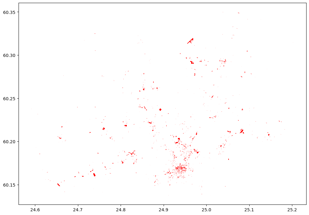
One handy trick and efficient trick for spatial join is to use it for selecting data. We can e.g. select all buildings that intersect with restaurants by conducting the spatial join other way around, i.e. using the buildings as the left GeoDataFrame and the restaurants as the right GeoDataFrame:

# Merge information from restaurants to buildings (conducts selection at the same time)
join2 = gpd.sjoin(buildings, restaurants, how="inner", op="intersects")
join2.plot()

/home/hentenka/.conda/envs/mamba/envs/sp-test/lib/python3.9/site-packages/IPython/core/interactiveshell.py:3318: FutureWarning: The `op` parameter is deprecated and will be removed in a future release. Please use the `predicate` parameter instead.
  if await self.run_code(code, result, async_=asy):

<AxesSubplot: >

As we can see (although the small building geometries are a bit poorly visible), the end result is a layer of buildings which intersected with the restaurants. This is a straightforward way to conduct simple spatial queries. You can specify with op parameter whether the binary predicate between the layers (i.e. the spatial relation between geometries) should be:

• intersects

• contains

• within

Plotting data with matplotlib

Thus far, we haven’t really made any effort to make our maps visually appealing. Let’s next see how we can adjust the appearance of our map, and how we can visualize many layers on top of each other. Let’s start by visualizing the buildings that we selected earlier and adjust a bit of the colors and figuresize. We can adjust the color of polygons with facecolor parameter and the figure size with figsize parameter that accepts a tuple of width and height as an argument:

ax = join2.plot(facecolor="red", figsize=(12,12))

join2.columns

Index(['addr:city_left', 'addr:country_left', 'addr:full',
       'addr:housenumber_left', 'addr:housename_left', 'addr:postcode_left',
       'addr:place_left', 'addr:street_left', 'email_left', 'name_left',
       'opening_hours_left', 'operator_left', 'phone_left', 'ref_left',
       'url_left', 'website_left', 'building_left', 'amenity_left',
       'building:flats', 'building:levels_left', 'building:material',
       'building:min_level', 'building:use', 'craft', 'height',
       'internet_access_left', 'landuse', 'levels', 'office_left', 'shop',
       'source_left', 'start_date_left', 'wikipedia_left', 'id_left',
       'timestamp_left', 'version_left', 'tags_left', 'osm_type_left',
       'geometry', 'changeset_left', 'index_right', 'version_right',
       'changeset_right', 'timestamp_right', 'id_right', 'lat', 'tags_right',
       'lon', 'addr:city_right', 'addr:country_right',
       'addr:housenumber_right', 'addr:housename_right', 'addr:postcode_right',
       'addr:place_right', 'addr:street_right', 'email_right', 'name_right',
       'opening_hours_right', 'operator_right', 'phone_right', 'ref_right',
       'url_right', 'website_right', 'amenity_right', 'bar', 'cafe',
       'drinking_water', 'internet_access_right', 'office_right', 'pub',
       'restaurant', 'source_right', 'start_date_right', 'wikipedia_right',
       'osm_type_right', 'building_right', 'building:levels_right'],
      dtype='object')

Now with the bigger figure size, it is already a bit easier to see the selected buildings that have a restaurant inside them (according OSM). Let’s color our buildings based on the building type. Hence, each building type category will receive a different color:

ax = join2.plot(column="building_left", cmap="RdYlBu", figsize=(12,12), legend=True)

Now we used the parameter column to specify the attribute that is used to specify the color for each building (can be categorical or continuous). We used cmap to specify the colormap for the categories and we added the legend by specifying legend=True. It is still a bit tricky to see what happens in our map. Luckily it is easy to zoom in to our map by using a specific commands (set_xlim() and set_ylim() that control the axis of our visualization:

# Zoom into city center by specifying X and Y coordinate extent
# These values should be given in the units that our data is presented (here decimal degrees)
xmin, xmax = 24.92, 24.98
ymin, ymax = 60.15, 60.18

# Plot the map again
ax = join2.plot(column="building_left", cmap="RdYlBu", figsize=(12,12), legend=True)

# Control and set the x and y limits for the axis
ax.set_xlim([xmin, xmax])
ax.set_ylim([ymin, ymax])

(60.15, 60.18)

Now it is much easier to see how the building types are distributed in the city. To get a bit more context to our visualizaton. Let’s also add roads with our buildings. To do that we first need to extract the roads from OSM:

# Get roads (retrieves walkable roads by default)
roads = osm.get_network()

Now we can continue and add the roads as a layer to our visualization with gray line color:

# Zoom into city center by specifying X and Y coordinate extent
# These values should be given in the units that our data is presented (here decimal degrees)
xmin, xmax = 24.92, 24.98
ymin, ymax = 60.15, 60.18

# Plot the map again
ax = join2.plot(column="building_left", cmap="RdYlBu", figsize=(12,12), legend=True)

# Plot the roads into the same axis
ax = roads.plot(ax=ax, edgecolor="gray", linewidth=0.75)

# Control and set the x and y limits for the axis
ax.set_xlim([xmin, xmax])
ax.set_ylim([ymin, ymax])

(60.15, 60.18)

Perfect! Now it is much easier to understand our map because the roads brought much more context (assuming you know Helsinki). We ware able to add the roads to the same map by specifying the ax parameter to point to the axis that we received when first plotting the join2 (i.e. selected buildings). In a similar manner, you can add as many layers in your map as you wish. Let’s still do a small visual trick and specify that the background color in our map is black instead of white. This can be done easily by changing the style of matplotlib visualization renderer:

# Import matplotlib pyplot and use a dark_background theme
import matplotlib.pyplot as plt
plt.style.use("dark_background")

# Zoom into city center by specifying X and Y coordinate extent
# These values should be given in the units that our data is presented (here decimal degrees)
xmin, xmax = 24.92, 24.98
ymin, ymax = 60.15, 60.18

# Plot the map again
ax = join2.plot(column="building_left", cmap="RdYlBu", figsize=(12,12), legend=True)

# Plot the roads into the same axis
ax = roads.plot(ax=ax, edgecolor="gray", linewidth=0.75)

# Control and set the x and y limits for the axis
ax.set_xlim([xmin, xmax])
ax.set_ylim([ymin, ymax])

(60.15, 60.18)

Awesome! Now we have a nice dark theme with our map. With this information you should be able to get going with Exercise 1.

Further information

For further information, we recommend checking the materials from Automating GIS Processes -course (GIS things) and Geo-Python -course (intro to Python and data analysis with pandas). In addition, we always recommend to check the latest documentation from the websites of the libraries:

• geopandas

• pyrosm

• matplotlib

• pandas