Tutorial 2.2: Spatial accessibility modelling with r5py

Credits:

This tutorial was written by Henrikki Tenkanen, Christoph Fink & Willem Klumpenhouwer (i.e. r5py developer team). You can read the full documentation of r5py which includes much more information and detailed user manual in case you are interested in using the library for research purposes.

Getting started

There are basically three options to run the codes in this tutorial:

1. Copy-Paste the codes from the website and run the codes line-by-line on your own computer with your preferred IDE (Jupyter Lab, Spyder, PyCharm etc.).

2. Download this Notebook (see below) and run it using Jupyter Lab which you should have installed by following the installation instructions.

3. Run the codes using Binder (see below) which is the easiest way, but has very limited computational resources (i.e. can be very slow).

Download the Notebook

You can download this tutorial Notebook to your own computer by clicking the Download button from the Menu on the top-right section of the website.

• Right-click the option that says .ipynb and choose “Save link as ..”

Run the codes on your own computer

Before you can run this Notebook, and/or do any programming, you need to launch the Jupyter Lab programming environment. The JupyterLab comes with the environment that you installed earlier (if you have not done this yet, follow the installation instructions). To run the JupyterLab:

1. Using terminal/command prompt, navigate to the folder where you have downloaded the Jupyter Notebook tutorial: $ cd /mydirectory/

2. Activate the programming environment: $ conda activate geo

3. Launch the JupyterLab: $ jupyter lab

After these steps, the JupyterLab interface should open, and you can start executing cells (see hints below at “Working with Jupyter Notebooks”).

Alternatively: Run codes in Binder (with limited resources)

Alternatively (not recommended due to limited computational resources), you can run this Notebook by launching a Binder instance. You can find buttons for activating the python environment at the top-right of this page which look like this:

Working with Jupyter Notebooks

Jupyter Notebooks are documents that can be used and run inside the JupyterLab programming environment containing the computer code and rich text elements (such as text, figures, tables and links).

A couple of hints:

• You can execute a cell by clicking a given cell that you want to run and pressing Shift + Enter (or by clicking the “Play” button on top)

• You can change the cell-type between Markdown (for writing text) and Code (for writing/executing code) from the dropdown menu above.

See further details and help for using Notebooks and JupyterLab from here.

Introduction

R5py is a Python library for routing and calculating travel time matrices on multimodal transport networks (walk, bike, public transport and car). It provides a simple and friendly interface to R⁵ (the Rapid Realistic Routing on Real-world and Reimagined networks) which is a routing engine developed by Conveyal. R5py is designed to interact with GeoPandas GeoDataFrames, and it is inspired by r5r which is a similar wrapper developed for R. R5py exposes some of R5’s functionality via its Python API, in a syntax similar to r5r’s. At the time of this writing, only the computation of travel time matrices has been fully implemented. Over time, r5py will be expanded to incorporate other functionalities from R5.

Data requirements

Data for creating a routable network

When calculating travel times with r5py, you typically need a couple of datasets:

• A road network dataset from OpenStreetMap (OSM) in Protocolbuffer Binary (.pbf) -format:

  • This data is used for finding the fastest routes and calculating the travel times based on walking, cycling and driving. In addition, this data is used for walking/cycling legs between stops when routing with transit.

  • Hint: Sometimes you might need modify the OSM data beforehand, e.g. by cropping the data or adding special costs for travelling (e.g. for considering slope when cycling/walking). When doing this, you should follow the instructions at Conveyal website. For adding customized costs for pedestrian and cycling analyses, see this repository.

• A transit schedule dataset in General Transit Feed Specification (GTFS.zip) -format (optional):

  • This data contains all the necessary information for calculating travel times based on public transport, such as stops, routes, trips and the schedules when the vehicles are passing a specific stop. You can read about GTFS standard from here.

  • Hint: r5py can also combine multiple GTFS files, as sometimes you might have different GTFS feeds representing e.g. the bus and metro connections.

Data for origin and destination locations

In addition to OSM and GTFS datasets, you need data that represents the origin and destination locations (OD-data) for routings. This data is typically stored in one of the geospatial data formats, such as Shapefile, GeoJSON or GeoPackage. As r5py is build on top of geopandas, it is easy to read OD-data from various different data formats.

Where to get these datasets?

Here are a few places from where you can download the datasets for creating the routable network:

• OpenStreetMap data in PBF-format:

  • pyrosm -library. Allows downloading data directly from Python (based on GeoFabrik and BBBike).

  • pydriosm -library. Allows downloading data directly from Python (based on GeoFabrik and BBBike).

  • GeoFabrik -website. Has data extracts for many pre-defined areas (countries, regions, etc).

  • BBBike -website. Has data extracts readily available for many cities across the world. Also supports downloading data by specifying your own area or interest.

  • Protomaps -website. Allows to download the data with custom extent by specifying your own area of interest.

• GTFS data:

  • Transitfeeds -website. Easy to navigate and find GTFS data for different countries and cities. Includes current and historical GTFS data. Notice: The site will be depracated in the future.

  • Mobility Database -website. Will eventually replace TransitFeeds -website.

  • Transitland -website. Find data based on country, operator or feed name. Includes current and historical GTFS data.

Sample datasets

In the following tutorial, we use various open source datasets:

• The point dataset for Helsinki has been obtained from Helsinki Region Environmental Services (HSY) licensed under a Creative Commons By Attribution 4.0.

• The street network for Helsinki is a cropped and filtered extract of OpenStreetMap (© OpenStreetMap contributors, ODbL license)

• The GTFS transport schedule dataset for Helsinki is a cropped and minimised copy of Helsingin seudun liikenne’s (HSL) open dataset Creative Commons BY 4.0.

Getting started with r5py

In this tutorial, we will learn how to calculate travel times with r5py between locations spread around the city center area of Helsinki, Finland.

Load and prepare the origin and destination data

Let’s start by downloading a sample dataset into a geopandas GeoDataFrame that we can use as our destination locations. To make testing the library easier, we have prepared a helper r5py.sampledata.helsinki which can be used to easily download the sample data sets for Helsinki (including population grid, GTFS data and OSM data). The population grid data covers the city center area of Helsinki and contains information about residents of each 250 meter cell:

import geopandas as gpd
import osmnx as ox
import r5py.sampledata.helsinki

pop_grid_fp = r5py.sampledata.helsinki.population_grid
pop_grid = gpd.read_file(pop_grid_fp)
pop_grid.head()

	id	population	geometry
0	0	389	POLYGON ((24.90545 60.16086, 24.90545 60.16311...
1	1	296	POLYGON ((24.90546 60.15862, 24.90545 60.16086...
2	2	636	POLYGON ((24.90547 60.15638, 24.90546 60.15862...
3	3	1476	POLYGON ((24.90547 60.15413, 24.90547 60.15638...
4	4	23	POLYGON ((24.90994 60.16535, 24.90994 60.16760...

The pop_grid GeoDataFrame contains a few columns, namely id, population and geometry. The id column with unique values and geometry columns are required for r5py to work. If your input dataset does not have an id column with unique values, r5py will throw an error.

To get a better sense of the data, let’s create a map that shows the locations of the polygons and visualise the number of people living in each cell:

pop_grid.explore("population", cmap="Reds")

Make this Notebook Trusted to load map: File -> Trust Notebook

Convert polygon layer to points

Lastly, we need to convert the Polygons into points because r5py expects that the input data is represented as points. We can do this by making a copy of our grid and calculating the centroid of the Polygons.

Note: You can ignore the UserWarning raised by geopandas about the geographic CRS. The location of the centroid is accurate enough for most purposes.

# Convert polygons into points
points = pop_grid.copy()
points["geometry"] = points.centroid
points.explore(max_zoom=13, color="red")

/tmp/ipykernel_52712/415363510.py:3: UserWarning: Geometry is in a geographic CRS. Results from 'centroid' are likely incorrect. Use 'GeoSeries.to_crs()' to re-project geometries to a projected CRS before this operation.

  points["geometry"] = points.centroid

Make this Notebook Trusted to load map: File -> Trust Notebook

Retrieve the origin location by geocoding an address

Let’s geocode an address for Helsinki Railway Station into a GeoDataFrame using osmnx and use that as our origin location:

from shapely.geometry import Point 

address = "Railway station, Helsinki, Finland"
lat, lon = ox.geocode(address)

# Create a GeoDataFrame out of the coordinates
origin = gpd.GeoDataFrame({"geometry": [Point(lon, lat)], "name": "Helsinki Railway station", "id": [0]}, index=[0], crs="epsg:4326")
origin.explore(max_zoom=13, color="red", marker_kwds={"radius": 12})

Make this Notebook Trusted to load map: File -> Trust Notebook

Load transport network

Virtually all operations of r5py require a transport network. In this example, we use data from Helsinki metropolitan area, which you can easily obtain from the r5py.sampledata.helsinki library. The files will be downloaded automatically to a temporary folder on your computer when you call the variables *.osm_pbf and *.gtfs:

# Download OSM data
r5py.sampledata.helsinki.osm_pbf

DataSet('/home/hentenka/.cache/r5py/kantakaupunki.osm.pbf')

# Download GTFS data
r5py.sampledata.helsinki.gtfs

DataSet('/home/hentenka/.cache/r5py/helsinki_gtfs.zip')

To import the street and public transport networks, instantiate an r5py.TransportNetwork with the file paths to the OSM extract and the GTFS files:

from r5py import TransportNetwork

# Get the filepaths to sample data (OSM and GTFS)
helsinki_osm = r5py.sampledata.helsinki.osm_pbf
helsinki_gtfs = r5py.sampledata.helsinki.gtfs

transport_network = TransportNetwork(
    # OSM data
    helsinki_osm,
    
    # A list of GTFS file(s)
    [
        helsinki_gtfs
    ]
)

At this stage, r5py has created the routable transport network and it is stored in the transport_network variable. We can now start using this network for doing the travel time calculations.

Info regarding “An illegal reflective access operation has occurred”

If you receive a Warning when running the cell above (“WARNING: An illegal reflective access operation has occurred”), it is due to using an older version of OpenJDK library (version 11). r5r only supports the version 11 of OpenJDK at this stage which is the reason why we also use it here. If you plan to use only r5py and want to get rid of the warning, you can update the OpenJDK to it’s latest version with mamba:

$ conda activate geo

$ mamba install -c conda-forge openjdk=20

Compute travel time matrix from one to all locations

A travel time matrix is a dataset detailing the travel costs (e.g., time) between given locations (origins and destinations) in a study area. To compute a travel time matrix with r5py based on public transportation, we first need to initialize an r5py.TravelTimeMatrixComputer -object. As inputs, we pass following arguments for the TravelTimeMatrixComputer:

• transport_network, which we created in the previous step representing the routable transport network.

• origins, which is a GeoDataFrame with one location that we created earlier (however, you can also use multiple locations as origins).

• destinations, which is a GeoDataFrame representing the destinations (in our case, the points GeoDataFrame).

• departure, which should be Python’s datetime -object (in our case standing for “22nd of February 2022 at 08:30”) to tell r5py that the schedules of this specific time and day should be used for doing the calculations.

  • Note: By default, r5py summarizes and calculates a median travel time from all possible connections within 10 minutes from given depature time (with 1 minute frequency). It is possible to adjust this time window using departure_time_window -parameter (see details here). For robust spatial accessibility assessment (e.g. in scientific works), we recommend to use 60 minutes departure_time_window.

• transport_modes, which determines the travel modes that will be used in the calculations. These can be passed using the options from the r5py.TransportMode -class.

  • Hint: To see all available options, run help(r5py.TransportMode).

Note

In addition to these ones, the constructor also accepts many other parameters listed here, such as walking and cycling speed, maximum trip duration, maximum number of transit connections used during the trip, etc.

Now, we will first create a travel_time_matrix_computer instance as described above:

import datetime
from r5py import TravelTimeMatrixComputer, TransportMode

# Initialize the tool
travel_time_matrix_computer = TravelTimeMatrixComputer(
    transport_network,
    origins=origin,
    destinations=points,
    departure=datetime.datetime(2022,2,22,8,30),
    transport_modes=[TransportMode.TRANSIT, TransportMode.WALK]
)

# To see all available transport modes, uncomment following
# help(TransportMode)

Running this initializes the TravelTimeMatrixComputer, but any calculations were not done yet. To actually run the computations, we need to call .compute_travel_times() on the instance, which will calculate the travel times between all points:

travel_time_matrix = travel_time_matrix_computer.compute_travel_times()
travel_time_matrix.head()

	from_id	to_id	travel_time
0	0	0	19
1	0	1	21
2	0	2	22
3	0	3	25
4	0	4	21

As a result, this returns a pandas.DataFrame which we stored in the travel_time_matrix -variable. The values in the travel_time column are travel times in minutes between the points identified by from_id and to_id. As you can see, the id value in the from_id column is the same for all rows because we only used one origin location as input.

To get a better sense of the results, let’s create a travel time map based on our results. We can do this easily by making a table join between the pop_grid GeoDataFrame and the travel_time_matrix. The key in the travel_time_matrix table is the column to_id and the corresponding key in pop_grid GeoDataFrame is the column id. Notice that here we do the table join with the original the Polygons layer (for visualization purposes). However, the join could also be done in a similar manner with the points GeoDataFrame.

join = pop_grid.merge(travel_time_matrix, left_on="id", right_on="to_id")
join.head()

	id	population	geometry	from_id	to_id	travel_time
0	0	389	POLYGON ((24.90545 60.16086, 24.90545 60.16311...	0	0	19
1	1	296	POLYGON ((24.90546 60.15862, 24.90545 60.16086...	0	1	21
2	2	636	POLYGON ((24.90547 60.15638, 24.90546 60.15862...	0	2	22
3	3	1476	POLYGON ((24.90547 60.15413, 24.90547 60.15638...	0	3	25
4	4	23	POLYGON ((24.90994 60.16535, 24.90994 60.16760...	0	4	21

Now we have the travel times attached to each point, and we can easily visualize them on a map:

m = join.explore("travel_time", cmap="Greens", max_zoom=13)
m = origin.explore(m=m, color="red", marker_kwds={"radius": 10})
m

Make this Notebook Trusted to load map: File -> Trust Notebook

Compute travel time matrix from all to all locations

Running the calculations between all points in our sample dataset can be done in a similar manner as calculating the travel times from one origin to all destinations. Since, calculating these kind of all-to-all travel time matrices is quite typical when doing accessibility analyses, it is actually possible to calculate a cross-product between all points just by using the origins parameter (i.e. without needing to specify a separate set for destinations). r5py will use the same points as destinations and produce a full set of origins and destinations:

travel_time_matrix_computer = TravelTimeMatrixComputer(
    transport_network,
    origins=points,
    departure=datetime.datetime(2022,2,22,8,30),
    transport_modes=[TransportMode.TRANSIT, TransportMode.WALK]
)
travel_time_matrix_all = travel_time_matrix_computer.compute_travel_times()
travel_time_matrix_all.head()

	from_id	to_id	travel_time
0	0	0	0
1	0	1	7
2	0	2	10
3	0	3	18
4	0	4	13

travel_time_matrix_all.tail()

	from_id	to_id	travel_time
8459	91	87	27
8460	91	88	23
8461	91	89	10
8462	91	90	6
8463	91	91	0

len(travel_time_matrix_all)

8464

As we can see from the outputs above, now we have calculated travel times between all points (n=92) in the study area. Hence, the resulting DataFrame has almost 8500 rows (92x92=8464). Based on these results, we can for example calculate the median travel time to or from a certain point, which gives a good estimate of the overall accessibility of the location in relation to other points:

median_times = travel_time_matrix_all.groupby("from_id")["travel_time"].median()
median_times

from_id
0     22.0
1     25.0
2     27.0
3     28.0
4     26.0
      ... 
87    25.0
88    25.0
89    23.0
90    26.0
91    28.0
Name: travel_time, Length: 92, dtype: float64

To estimate, how long does it take in general to travel between locations in our study area (i.e. what is the baseline accessibility in the area), we can calculate the mean (or median) of the median travel times showing that it is approximately 22 minutes:

median_times.mean()

21.918478260869566

Naturally, we can also visualize these values on a map:

overall_access = pop_grid.merge(median_times.reset_index(), left_on="id", right_on="from_id")
overall_access.head()

	id	population	geometry	from_id	travel_time
0	0	389	POLYGON ((24.90545 60.16086, 24.90545 60.16311...	0	22.0
1	1	296	POLYGON ((24.90546 60.15862, 24.90545 60.16086...	1	25.0
2	2	636	POLYGON ((24.90547 60.15638, 24.90546 60.15862...	2	27.0
3	3	1476	POLYGON ((24.90547 60.15413, 24.90547 60.15638...	3	28.0
4	4	23	POLYGON ((24.90994 60.16535, 24.90994 60.16760...	4	26.0

overall_access.explore("travel_time", cmap="Blues", scheme="natural_breaks", k=4)

Make this Notebook Trusted to load map: File -> Trust Notebook

In out study area, there seems to be a bit poorer accessibility in the Southern areas and on the edges of the region (i.e. we wittness a classic edge-effect here).

Advanced usage

Compute travel times with a detailed information about the routing results

In case you are interested in more detailed routing results, it is possible to use DetailedItinerariesComputer. This will provide not only the same information as in the previous examples, but it also brings much more detailed information about the routings. When using this functionality, r5py produces information about the used routes for each origin-destination pair (with possibly multiple alternative routes), as well as individual trip segments and information about the used modes, public transport route-id information (e.g. bus-line number), distanes, waiting times and the actual geometry used.

Important

Computing detailed itineraries is significantly more time-consuming than calculating simple travel times. As such, think twice whether you actually need the detailed information output from this function, and how you might be able to limit the number of origins and destinations you need to compute.

from r5py import DetailedItinerariesComputer

# Take a small sample of destinations for demo purposes
points_sample = points.sample(3)

travel_time_matrix_computer = DetailedItinerariesComputer(
    transport_network,
    origins=origin,
    destinations=points_sample,
    departure=datetime.datetime(2022,2,22,8,30),
    transport_modes=[TransportMode.TRANSIT, TransportMode.WALK],
    
    # With following attempts to snap all origin and destination points to the transport network before routing
    snap_to_network=True,
)
travel_details = travel_time_matrix_computer.compute_travel_details()
travel_details.head()

/home/hentenka/.conda/envs/mamba/envs/geo/lib/python3.11/site-packages/r5py/r5/detailed_itineraries_computer.py:135: RuntimeWarning: R5 has been compiled with `TransitLayer.SAVE_SHAPES = false` (the default). The geometries of public transport routes are inaccurate (straight lines between stops), and distances can not be computed.
  warnings.warn(

	from_id	to_id	option	segment	transport_mode	departure_time	distance	travel_time	wait_time	route	geometry
0	0	45	0	0	TransportMode.WALK	NaT	915.927	0 days 00:15:46	NaT	None	LINESTRING (24.94128 60.17285, 24.94143 60.171...
1	0	45	1	0	TransportMode.WALK	2022-02-22 08:38:53	228.424	0 days 00:03:55	0 days 00:00:00	None	LINESTRING (24.94128 60.17285, 24.94143 60.171...
2	0	45	1	1	TransportMode.TRAM	2022-02-22 08:46:00	NaN	0 days 00:03:00	0 days 00:03:21	9	LINESTRING (24.94061 60.17040, 24.93530 60.168...
3	0	45	1	2	TransportMode.WALK	2022-02-22 08:50:00	316.744	0 days 00:05:33	0 days 00:00:00	None	LINESTRING (24.93494 60.16635, 24.93478 60.166...
4	0	45	2	0	TransportMode.WALK	2022-02-22 08:35:37	256.017	0 days 00:04:21	0 days 00:00:00	None	LINESTRING (24.94128 60.17285, 24.94143 60.171...

As you can see, the result contains much more information than earlier, see the following table for explanations:

Column	Description	Data type
from_id	the origin of the trip this segment belongs to	any, user defined
to_id	the destination of the trip this segment belongs to	any, user defined
option	sequential number for different trip options found	int
segment	sequential number for segments of the current trip options	int
transport_mode	the transport mode used on the current segment	r5py.TransportMode
departure_time	the transit departure date and time used for current segment	datetime.datetime
distance	the travel distance in metres for the current segment	float
travel_time	The travel time for the current segment	datetime.timedelta
wait_time	The wait time between connections when using public transport	datetime.timedelta
route	The route number or id for public transport route used on a segment	str
geometry	The path travelled on a current segment (with transit, stops connected with straight lines by default)	shapely.LineString

Visualize the routes on a map

In the following, we will make a nice interactive visualization out of the results, that shows the fastest routes and the mode of transport between the given origin-destination pairs (with multiple alternative trips/routes):

import folium 
import folium.plugins

# Convert travel mode to string (from r5py.TransportMode object)
travel_details["mode"] = travel_details["transport_mode"].astype(str)

# Calculate travel time in minutes (from timedelta)
travel_details["travel time (min)"] = (travel_details["travel_time"].dt.total_seconds() / 60).round(2)

# Generate text for given trip ("origin" to "destination")
travel_details["trip"] = travel_details["from_id"].astype(str) + " to " + travel_details["to_id"].astype(str)

# Choose columns for visualization
selected_cols = ["geometry", "distance", "mode", "route", "travel time (min)", "trip", "from_id", "to_id", "option", "segment"  ]

# Generate the map
m = travel_details[selected_cols].explore(
    tooltip=["trip", "option", "segment", "mode", "route", "travel time (min)", "distance"],
    column="mode",
    tiles="CartoDB.Positron",
    )

# Add marker for the origin
m = origin.explore(m=m, marker_type="marker", marker_kwds=dict(icon=folium.Icon(color="green", icon="train", prefix="fa", )))

# Add customized markers for destinations
points_sample.apply(lambda row: (
        # Marker with destination ID number attached to the icon
        folium.Marker(
            (row["geometry"].y, row["geometry"].x),
            icon=folium.plugins.BeautifyIcon(
                icon_shape="marker",
                number=row["id"],
                border_color="#728224",
                text_color="#728224",
            )
        # Add the marker to existing map    
        ).add_to(m)), axis=1,
)

m

Make this Notebook Trusted to load map: File -> Trust Notebook

As a result, now we have a nice map that shows alternative routes between Railway station and the given destinations in the study area. If you hover over the lines, you can see details about the selected routes with useful information about the travel time, distance, route id (line number) etc. Hence, as such, if you’re feeling nerdy (and happen to have Python installed to your phone 😛), you could replace your Google Maps navigator or other journey planners with r5py! 🤓😉

Geometries of public transport routes, and distances travelled

The default version of R⁵ is configured for performance reasons in a way that it does not read the geometries included in GTFS data sets.

As a consequence, the geometry reported by DetailedItinerariesComputer are straight lines in-between the stops of a public transport line, and do not reflect the actual path travelled in public transport modes.

With this in mind, r5py does not attempt to compute the distance of public transport segments if SAVE_SHAPES = false, as distances would be very crude approximations, only. Instead it reports NaN/None.

The Digital Geography Lab maintains a patched version of R⁵ in its GitHub repositories. If you want to refrain from compiling your own R⁵ jar, but still would like to use detailed geometries of public transport routes, follow the instructions in Advanced use of r5py documentation.

Large-scale analyses - Travel time matrices covering massive number of connections

When trying to understand the accessibility of a specific location, you typically want to look at travel times between multiple locations (one-to-many). Next, we will learn how to calculate travel time matrices using r5py Python library.

When calculating travel times with r5py, you typically need a couple of datasets:

• A road network dataset from OpenStreetMap (OSM) in Protocolbuffer Binary (.pbf) format:

  • This data is used for finding the fastest routes and calculating the travel times based on walking, cycling and driving. In addition, this data is used for walking/cycling legs between stops when routing with transit.

  • Hint: Sometimes you might need modify the OSM data beforehand, e.g., by cropping the data or adding special costs for travelling (e.g., for considering slope when cycling/walking). When doing this, you should follow the instructions on the Conveyal website. For adding customized costs for pedestrian and cycling analyses, see this repository.

• A transit schedule dataset in General Transit Feed Specification (GTFS.zip) format (optional):

  • This data contains all the necessary information for calculating travel times based on public transport, such as stops, routes, trips and the schedules when the vehicles are passing a specific stop. You can read about the GTFS standard here.

  • Hint: r5py can also combine multiple GTFS files, as sometimes you might have different GTFS feeds representing, e.g., the bus and metro connections.

Sample data

In this tutorial, we use two datasets:

1. Helsinki.osm.pbf - Covers the OSM data for Helsinki Region (cities of Helsinki, Espoo, Vantaa, Kauniainen)

2. GTFS_Helsinki.zip - Covers the GTFS data for Helsinki Region.

Download the data for own computer (optional)

CLICK and Download the data covering Helsinki Metropolitan Area (90 MB). The ZIP file contains two files mentioned above.

Copy the data at CSC environment

Run the following command to copy the data files which makes it possible for you to start working with them:

!cp $HOME/shared/data/Helsinki/GTFS_Helsinki.zip $HOME/shared/data/Helsinki/Helsinki.osm.pbf /$HOME/notebooks/sustainability-gis/L2/data/Helsinki

Load the origin and destination data

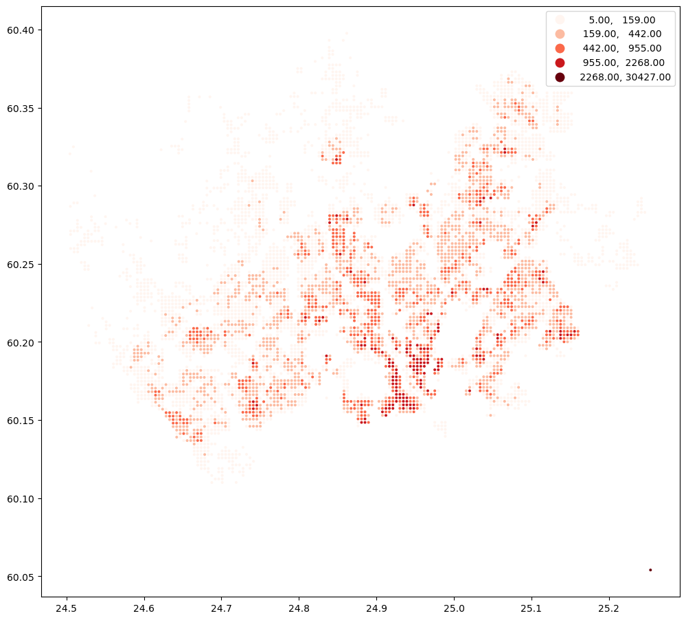
Let’s start by downloading a sample point dataset into a geopandas GeoDataFrame that we can use as our origin and destination locations. For the sake of this exercise, we have prepared a grid of points covering parts of Helsinki. The point data also contains the number of residents of each 250 meter cell:

import geopandas as gpd
import ssl

# Without the following you might get certificate error (at least on Linux)
ssl._create_default_https_context = ssl._create_unverified_context

# Calculate travel times to railway station from all grid cells
pop_grid_wfs = "https://kartta.hsy.fi/geoserver/wfs?request=GetFeature&typename=asuminen_ja_maankaytto:Vaestotietoruudukko_2021&outputformat=JSON"
pop_grid = gpd.read_file(pop_grid_wfs)

# Get centroids
points = pop_grid.copy()
points["geometry"] = points.centroid

# Reproject
points = points.to_crs(epsg=4326)
points.plot("asukkaita", scheme="natural_breaks", cmap="Reds", figsize=(12,12), legend=True, markersize=3.5)

<Axes: >

Next, we will geocode the address for Helsinki Railway station. For doing this, we can use oxmnx library and its handy .geocode() -function:

import osmnx as ox
from shapely.geometry import Point

# Find coordinates of the central railway station of Helsinki
lat, lon = ox.geocode("Rautatieasema, Helsinki")

# Create a GeoDataFrame out of the coordinates
station = gpd.GeoDataFrame({"geometry": [Point(lon, lat)], "name": "Helsinki Railway station", "id": [0]}, index=[0], crs="epsg:4326")
station.explore(max_zoom=13, color="red", marker_kwds={"radius": 12})

Make this Notebook Trusted to load map: File -> Trust Notebook

• Next, we will prepare the routable network in a similar fashion as before, but now we use the larger data files which we downloaded earlier.

import datetime
from r5py import TransportNetwork, TravelTimeMatrixComputer, TransportMode

# Filepath to OSM data
osm_fp = "data/Helsinki/Helsinki.osm.pbf"

transport_network = TransportNetwork(
    osm_fp,
    [
        "data/Helsinki/GTFS_Helsinki.zip"
    ]
)

• After this step, we can do the routing

travel_time_matrix_computer = TravelTimeMatrixComputer(
    transport_network,
    origins=station,
    destinations=points,
    departure=datetime.datetime(2022,8,15,8,30),
    transport_modes=[TransportMode.TRANSIT, TransportMode.WALK],
)
travel_time_matrix = travel_time_matrix_computer.compute_travel_times()

travel_time_matrix.head()

	from_id	to_id	travel_time
0	0	Vaestotietoruudukko_2021.1	90.0
1	0	Vaestotietoruudukko_2021.2	82.0
2	0	Vaestotietoruudukko_2021.3	79.0
3	0	Vaestotietoruudukko_2021.4	78.0
4	0	Vaestotietoruudukko_2021.5	86.0

• Now we can join the travel time information back to the population grid

geo = pop_grid.merge(travel_time_matrix, left_on="id", right_on="to_id")
geo.head()

	id	index	asukkaita	asvaljyys	ika0_9	ika10_19	ika20_29	ika30_39	ika40_49	ika50_59	ika60_69	ika70_79	ika_yli80	geometry	from_id	to_id	travel_time
0	Vaestotietoruudukko_2021.1	688	5	50.60	99	99	99	99	99	99	99	99	99	POLYGON ((25472499.995 6689749.005, 25472499.9...	0	Vaestotietoruudukko_2021.1	90.0
1	Vaestotietoruudukko_2021.2	703	7	36.71	99	99	99	99	99	99	99	99	99	POLYGON ((25472499.995 6685998.998, 25472499.9...	0	Vaestotietoruudukko_2021.2	82.0
2	Vaestotietoruudukko_2021.3	710	8	44.50	99	99	99	99	99	99	99	99	99	POLYGON ((25472499.995 6684249.004, 25472499.9...	0	Vaestotietoruudukko_2021.3	79.0
3	Vaestotietoruudukko_2021.4	711	7	64.14	99	99	99	99	99	99	99	99	99	POLYGON ((25472499.995 6683999.005, 25472499.9...	0	Vaestotietoruudukko_2021.4	78.0
4	Vaestotietoruudukko_2021.5	715	11	41.09	99	99	99	99	99	99	99	99	99	POLYGON ((25472499.995 6682998.998, 25472499.9...	0	Vaestotietoruudukko_2021.5	86.0

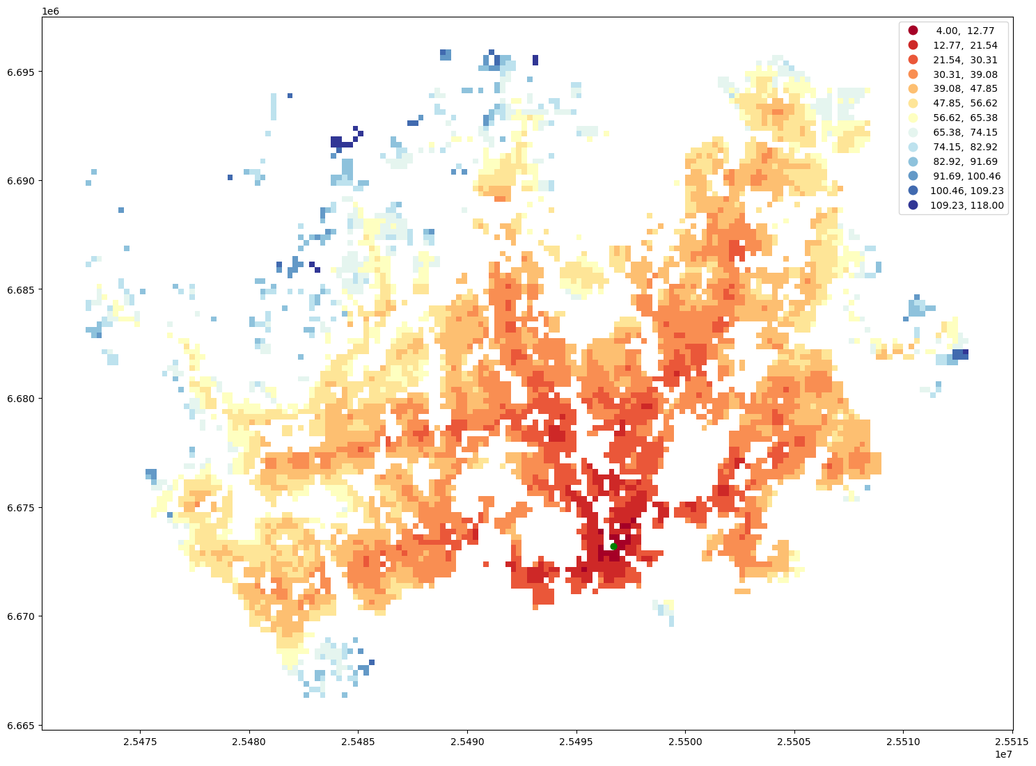
• Finally, we can visualize the travel time map and investigate how the railway station in Helsinki can be accessed from different parts of the region, by public transport.

ax = geo.plot(column="travel_time", cmap="RdYlBu", scheme="equal_interval", k=13, legend=True, figsize=(18,18))
ax = station.to_crs(crs=geo.crs).plot(ax=ax, color="green", markersize=40)

Calculate travel times by bike

In a very similar manner, we can calculate travel times by cycling. We only need to modify our TravelTimeMatrixComputer object a little bit. We specify the cycling speed by using the parameter speed_cycling and we change the transport_modes parameter to correspond to [TransportMode.WALK, TransportMode.BICYCLE]. This will initialize the object for cycling analyses:

tc_bike = TravelTimeMatrixComputer(
    transport_network,
    origins=station,
    destinations=points,
    speed_cycling=16,
    transport_modes=[TransportMode.WALK, TransportMode.BICYCLE],
)
ttm_bike = tc_bike.compute_travel_times()

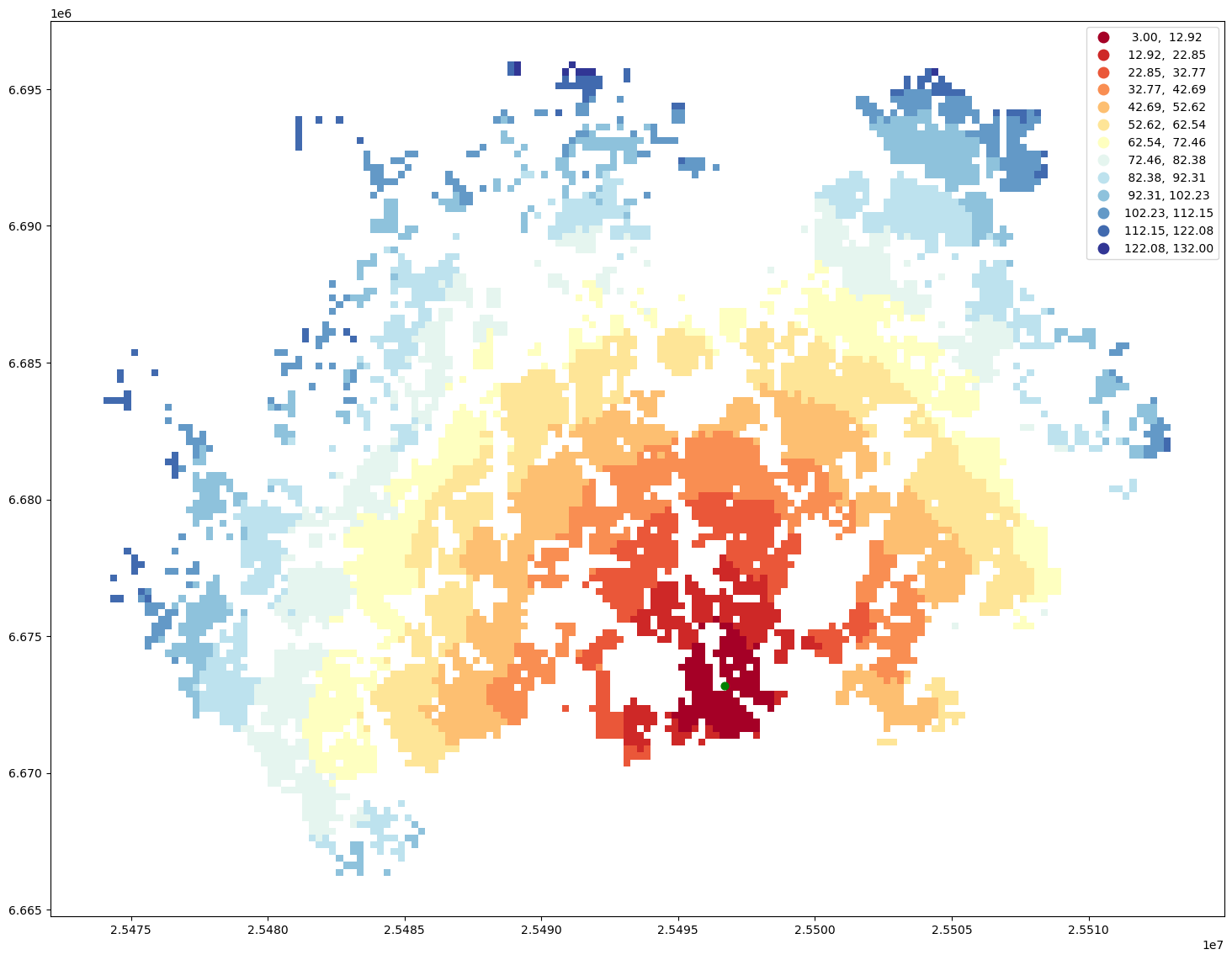
• Let’s again make a table join with the population grid and plot the data:

geo = pop_grid.merge(ttm_bike, left_on="id", right_on="to_id")
ax = geo.plot(column="travel_time", cmap="RdYlBu", scheme="equal_interval", k=13, legend=True, figsize=(18,18))
ax = station.to_crs(crs=geo.crs).plot(ax=ax, color="green", markersize=40)

Calculate catchment areas

One quite typical accessibility analysis is to find out catchment areas for multiple locations, such as libraries. In the below, we will extract all libraries in Helsinki region and calculate travel times from all grid cells to the closest one. As a result, we have catchment areas for each library.

• Let’s start by parsing the libraries in Helsinki region (covering four cities in the region), using osmnx:

import osmnx as ox

# Fetch libraries from multiple cities simultaneously
query = ["Helsinki, Finland", "Espoo, Finland", "Vantaa, Finland", "Kauniainen, Finland"]
libraries = ox.features_from_place(query, tags={"amenity": ["library"]})

# Show first rows
libraries.head()

		addr:city	addr:housenumber	addr:postcode	addr:street	amenity	internet_access	level	name	name:fi	name:sv	...	roof:shape	source:architect	source:start_date	name:da	building:part	air_conditioning	alt_name:ru	name:fr	name:ja	short_name
element_type	osmid
node	50807898	Helsinki	2	00880	Linnanrakentajantie	library	yes	1	Herttoniemen kirjasto	Herttoniemen kirjasto	Hertonäs bibliotek	...	NaN	NaN	NaN	NaN	NaN	NaN	NaN	NaN	NaN	NaN
	50821497	Helsinki	2	00820	Roihuvuorentie	library	NaN	NaN	Roihuvuoren kirjasto	Roihuvuoren kirjasto	Kasbergets bibliotek	...	NaN	NaN	NaN	NaN	NaN	NaN	NaN	NaN	NaN	NaN
	54043622	NaN	NaN	NaN	NaN	library	NaN	NaN	Viikin kirjasto	Viikin kirjasto	Viks bibliotek	...	NaN	NaN	NaN	NaN	NaN	NaN	NaN	NaN	NaN	NaN
	55891898	Kauniainen	6	02700	Thurmaninaukio	library	NaN	NaN	Kauniaisten kaupunginkirjasto	Kauniaisten kirjasto	Grankulla bibliotek	...	NaN	NaN	NaN	NaN	NaN	NaN	NaN	NaN	NaN	NaN
	60123861	Helsinki	4	00940	Ostostie	library	NaN	NaN	Kontulan kirjasto	Kontulan kirjasto	Gårdsbacka bibliotek	...	NaN	NaN	NaN	NaN	NaN	NaN	NaN	NaN	NaN	NaN

5 rows × 85 columns

• Some of the libraries might be in Polygon format, so we need to convert them into points by calculating their centroid:

# Convert the geometries to points
libraries["geometry"] = libraries.centroid

/tmp/ipykernel_52712/4134701274.py:2: UserWarning: Geometry is in a geographic CRS. Results from 'centroid' are likely incorrect. Use 'GeoSeries.to_crs()' to re-project geometries to a projected CRS before this operation.

  libraries["geometry"] = libraries.centroid

• Let’s see how the distribution of libraries looks on a map:

libraries.explore(color="red", marker_kwds=dict(radius=5))

Make this Notebook Trusted to load map: File -> Trust Notebook

# Ensure that every row have an unique id
libraries = libraries.reset_index()
libraries["id"] = libraries.index
libraries.head()

	element_type	osmid	addr:city	addr:housenumber	addr:postcode	addr:street	amenity	internet_access	level	name	...	source:architect	source:start_date	name:da	building:part	air_conditioning	alt_name:ru	name:fr	name:ja	short_name	id
0	node	50807898	Helsinki	2	00880	Linnanrakentajantie	library	yes	1	Herttoniemen kirjasto	...	NaN	NaN	NaN	NaN	NaN	NaN	NaN	NaN	NaN	0
1	node	50821497	Helsinki	2	00820	Roihuvuorentie	library	NaN	NaN	Roihuvuoren kirjasto	...	NaN	NaN	NaN	NaN	NaN	NaN	NaN	NaN	NaN	1
2	node	54043622	NaN	NaN	NaN	NaN	library	NaN	NaN	Viikin kirjasto	...	NaN	NaN	NaN	NaN	NaN	NaN	NaN	NaN	NaN	2
3	node	55891898	Kauniainen	6	02700	Thurmaninaukio	library	NaN	NaN	Kauniaisten kaupunginkirjasto	...	NaN	NaN	NaN	NaN	NaN	NaN	NaN	NaN	NaN	3
4	node	60123861	Helsinki	4	00940	Ostostie	library	NaN	NaN	Kontulan kirjasto	...	NaN	NaN	NaN	NaN	NaN	NaN	NaN	NaN	NaN	4

5 rows × 88 columns

• Next, we can initialize our travel time matrix calculator using the libraries as the origins:

travel_time_matrix_computer = TravelTimeMatrixComputer(
    transport_network,
    origins=libraries,
    destinations=points,
    departure=datetime.datetime(2022,8,15,8,30),
    transport_modes=[TransportMode.TRANSIT, TransportMode.WALK],
)
travel_time_matrix = travel_time_matrix_computer.compute_travel_times()

travel_time_matrix.shape

(538476, 3)

• As we can see, there are almost 540 thousand rows of data, which comes as a result of all connections between origins and destinations. Next, we want aggregate the data and keep only travel time information to the closest library:

# Find out the travel time to closest library
closest_library = travel_time_matrix.groupby("to_id")["travel_time"].min().reset_index()
closest_library

	to_id	travel_time
0	Vaestotietoruudukko_2021.1	57.0
1	Vaestotietoruudukko_2021.10	56.0
2	Vaestotietoruudukko_2021.100	50.0
3	Vaestotietoruudukko_2021.1000	28.0
4	Vaestotietoruudukko_2021.1001	32.0
...	...	...
5848	Vaestotietoruudukko_2021.995	20.0
5849	Vaestotietoruudukko_2021.996	17.0
5850	Vaestotietoruudukko_2021.997	20.0
5851	Vaestotietoruudukko_2021.998	38.0
5852	Vaestotietoruudukko_2021.999	33.0

5853 rows × 2 columns

Then we can make a table join with the grid in a similar manner as previously and visualize the data:

# Make a table join
geo = pop_grid.merge(closest_library, left_on="id", right_on="to_id")

# Visualize the data
ax = geo.plot(column="travel_time", cmap="RdYlBu", scheme="natural_breaks", k=10, legend=True, figsize=(18,18))
ax = station.to_crs(crs=geo.crs).plot(ax=ax, color="green", markersize=40)

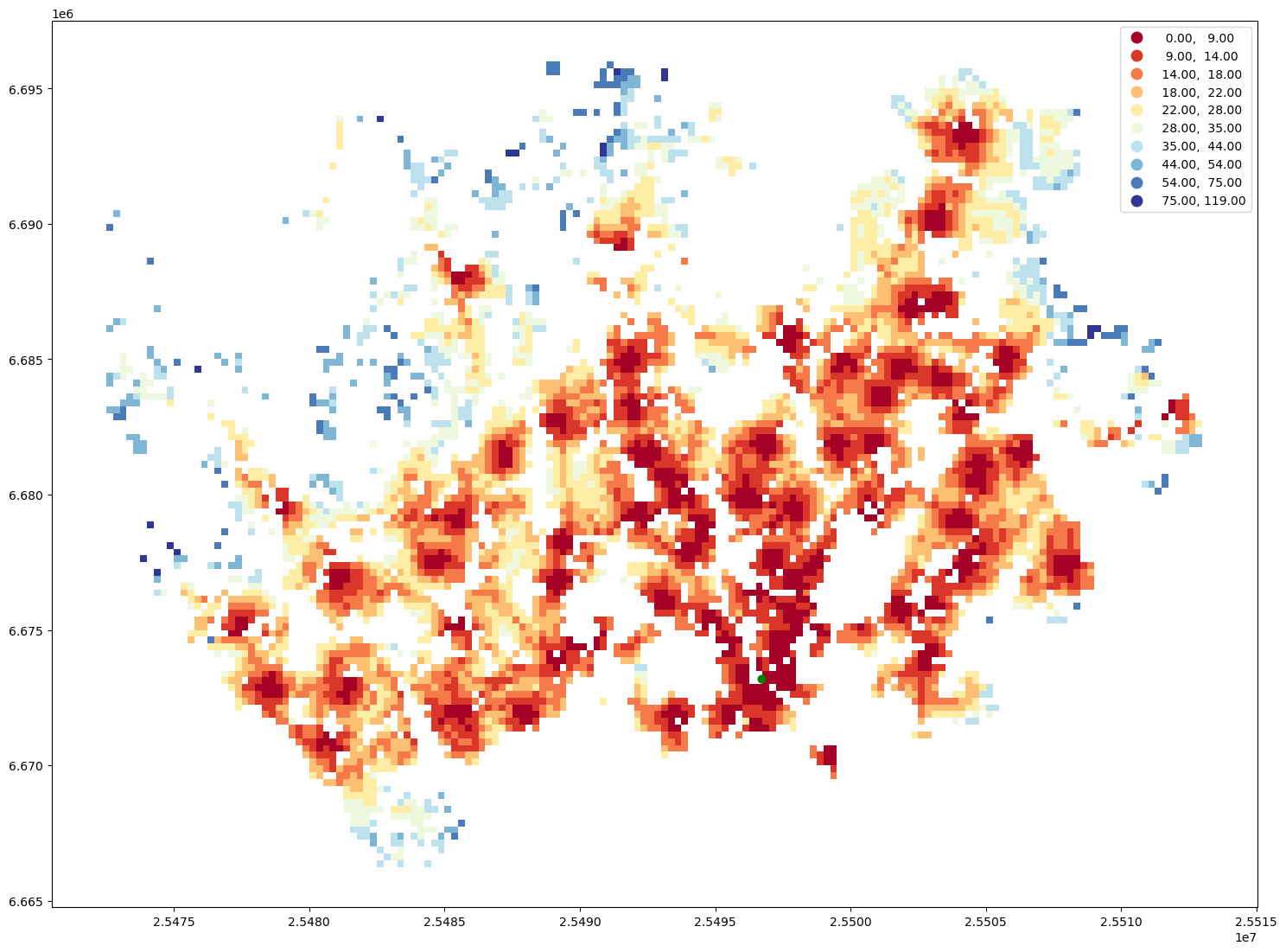
That’s it! As you can, see now we have a nice map showing the catchment areas for each library.

Analyze accessibility

After we have calculated the travel times to the closest services, we can start analyzing accessibility. There are various ways to analyze how accessible services are. Here, for the sake of simplicity, we calculate the number of inhabitants that can reach the services within given travel time thershold (e.g. 15 minutes) by PT (or walking).

# Extract the grid cells within given travel time threshold
threshold = 15
access = geo.loc[geo["travel_time"]<=threshold].copy()

ax = access.plot(column="asukkaita", figsize=(10,5), legend=True)
ax.set_title(f"The number of people living within {threshold} minutes travel time threshold.");

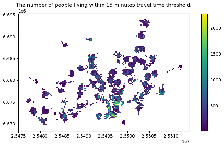
Now we can easily calculate how many people or what is the proportion of people that can access the given service within the given travel time threshold:

pop_within_threshold = access["asukkaita"].sum()
pop_share = pop_within_threshold / geo["asukkaita"].sum()
print(f"Population within accessibility thresholds: {pop_within_threshold} ({pop_share*100:.0f} %)")

Population within accessibility thresholds: 667457 (55 %)

We can see that approximately 55 % of the population in the region can access a library within given time threshold. With this information we can start evaluating whether the level of access for the population in the region can be considered as “sufficient” or equitable. Naturally, with more detailed data, we could start evaluating whether e.g. certain population groups have lower access than on average in the region, which enables us to start studying the questions of justice and equity. Often the interesting question is to understand “who does not have access”? I.e. who is left out.

There are many important questions relating to equity of access that require careful consideration when doing these kind of analyses is for example what is seen as “reasonable” level of access. I.e. what should be specify as the travel time threshold in our analysis. Answering to these kind of questions is not straightforward as the accessibility thresholds (i.e. travel time budget) are very context dependent and normative (value based) by nature.

Cumulative opportunities

Another commonly used approach to analyze accessibility is to analyze how many services can a given individual (or group of individuals) access within given travel time budget. This is called cumulative opportunities measure.

# How many services can be reached from each grid cell within given travel time threshold?
travel_time_matrix.head()

	from_id	to_id	travel_time
0	0	Vaestotietoruudukko_2021.1	117.0
1	0	Vaestotietoruudukko_2021.2	110.0
2	0	Vaestotietoruudukko_2021.3	107.0
3	0	Vaestotietoruudukko_2021.4	106.0
4	0	Vaestotietoruudukko_2021.5	100.0

threshold = 15
# Count the number of opportunities from each grid cell
opportunities = travel_time_matrix.loc[travel_time_matrix["travel_time"]<=threshold].groupby("to_id")["from_id"].count().reset_index()

# Rename the column for more intuitive one
opportunities = opportunities.rename(columns={"from_id": "num_opportunities"})

# Merge with population grid
opportunities = pop_grid.merge(opportunities, left_on="id", right_on="to_id")

# Plot the results
ax = opportunities.plot(column="num_opportunities", figsize=(10,5), legend=True)
ax.set_title(f"Number of opportunities within {threshold} minutes."); 

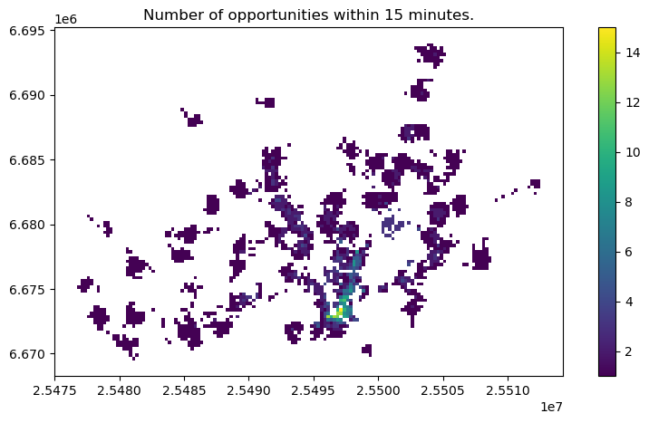
Now we can clearly see the areas with highest level of accessibility to given service. This is called cumulative opportunities measure or “Hansen’s Accessibility” measure after its developer.

At times one could still want apply a distance decay function to give more weight to the closer services and less to the services that are further away, and hence less likely to be visited by citizens who seek to use the service. This is called as time-weighted cumulative opportunities measure. There are also many other approaches to measure accessibility which are out of scope of this tutorial. In case you are interested in understanding more, I recommend reading following papers:

• Levinson, D. & H. Wu (2020). Towards a general theory of access.

• Wu, H. & D. Levinson (2020). Unifying access.

Where to go next?

In case you want to learn more, we recommend reading:

• r5py documentation that provides much more details on how to use r5py.